3. Introduction to Sampling Distributions — Runestone Interactive Overview

3.1. Evaluating Studies¶

In class, we conducted some simulations to identity the effect of the first of two forms of randomization, randomized selection of individual units. Based on these activities, we identified two main effects of randomization.

The effect of random selection of individuals in sampling

Using a random sampling technique to select individuals resulted in unbiased estimates of parameters. In other words, our statistics did not tend to over- or under-estimate the parameter, but balanced these errors instead. (This assumes no other source of bias.)

When evaluating a statistical study, the first thing that should be considered is the appropriate scope of the conclusions, that is to say the types of conclusions that are justified for this type of study. The following table gives some advice on what conclusions can be drawn based on whether or not there was random sampling.

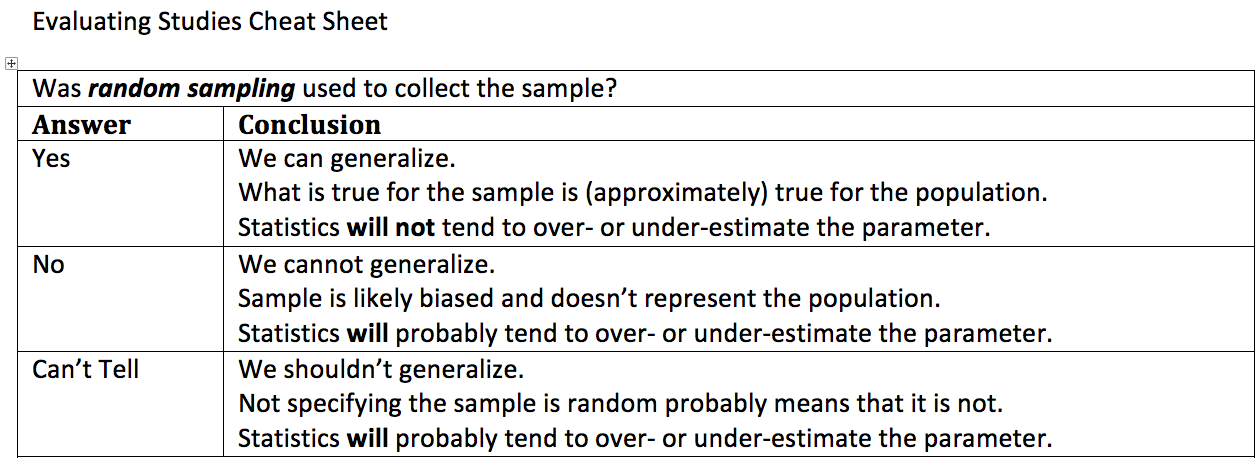
Evaluating studies cheat sheet

A study on flossing and gum disease (experiment)

A recent study was conducted to determine the effectiveness of flossing on gum disease. A group of 500 volunteers were randomly split into two groups. The first group was asked to floss once a day and the second group was asked to floss after each meal. Suppose that the group that flossed after every meal was much less likely to have gum disease as the group that flossed once per day.

(A) Yes
Note that the description mentioned that the participants were volunteers.
(B) No
The participants volunteered and were not randomly selected.

(A) Yes, the effects the flossing treatments would be the same for the general population.
The participants in the study were volunteers and not a randomly selected sample.
(B) No, there is a danger that our estimates of the effects of flossing on gum disease is likely biased.
The lack of a randomly selected sample means that we are in danger of biased estimates.

Another study on flossing and gum disease (observational study)

In another study on flossing and gum disease, a random sample of 500 people were surveyed on their flossing habits and whether or not they suffered from gum disease. Suppose that it was estimated that the people that flossed after every meal was much less likely to have gum disease as the group that flossed once per day.

(A) Yes
(B) No
The text explicitly mentioned a random sample.

(A) Yes, the effects the flossing treatments will be the same for the general population.
Because we are taking a random sample, our statistics should be unbiased and not over- or under-estimate the rates of gum disease in each group.
(B) No, there is a danger that our estimates of the effects of flossing on gum disease is likely biased.
What is the effect of random sampling on bias and a statistics ability to estimate a parameter?

3.2. Overview of Statistical Inference¶

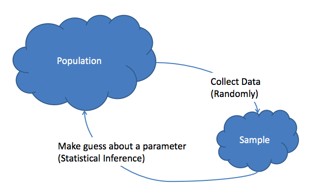
When asking questions about some population of individuals, the ideal situation is collecting information on all of the individuals of interest. This is referred to as taking a census of the population. Most of the time, it is not feasible to collect information on the entire population. In this case, we collect data on a sample of the population and use this information to make educated guesses about the population. This is referred to as statistical inference. More specifically, in statistical inference, we use sample statistics to make inferences (guesses) about population parameters.

Statistical Inference: The process of making educated guess about population parameters using information collected from a random sample, e.g. a sample statistic.

Note

The federal government of the United States takes a “census” every 10 years, but there are a number of reasons this census falls short of the statistical definition.

The population is defined over households not individual citizens.
The Census Bureau only attempts to collect a small amount of information on all households. The long form is collected on a sample of households.
There is a fraction of the population for which it is nearly impossible to survey

3.2.1. Notation for Parameters and Statistics¶

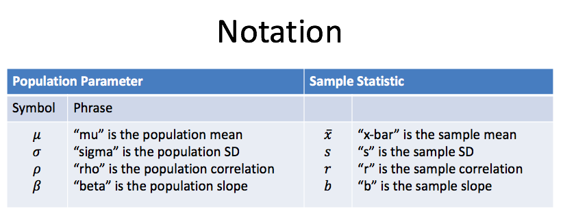
In statistics there is a very big distinction between parameters (number describing a population) and statistics (numbers describing a sample).

Distinction between Parameters and Statistics

Parameters are thought of as the exact values that we would like to make guesses about. They are generally too expensive to find exactly and are almost always unknown.
Statistics are thought of as a guess of the value of a parameter. They are not particularly interesting in their own right.

The difference between parameters and statistics is so important that we use different symbols to represent each. The first summary method that we will focus on is the mean or average of quantitative data. The symbol that we use for a population mean (parameter) is \(\mu\), while the symbol we use for a sample mean (statistic) is \(\bar{x}\). The following table gives the symbols for various parameters and statistics we will work within this course.

3.3. Sampling Distributions¶

The first and most important fact that you need to realize when working with statistics is statistics vary from sample to sample. This is known as sampling variability and most of the procedures in statistics are methods for dealing with sampling variability.

Sampling Variability: Sampling variability refers to the natural variation in statistics taken from different samples. It is very important to quantify this variability.
Standard Error: The standard error is the estimated standard deviation of the sample statistics. It is an important measure of sampling variability.

To get an idea of the typical location of and variability between: sample statistics (i.e. center and spread), we study the sampling distribution.

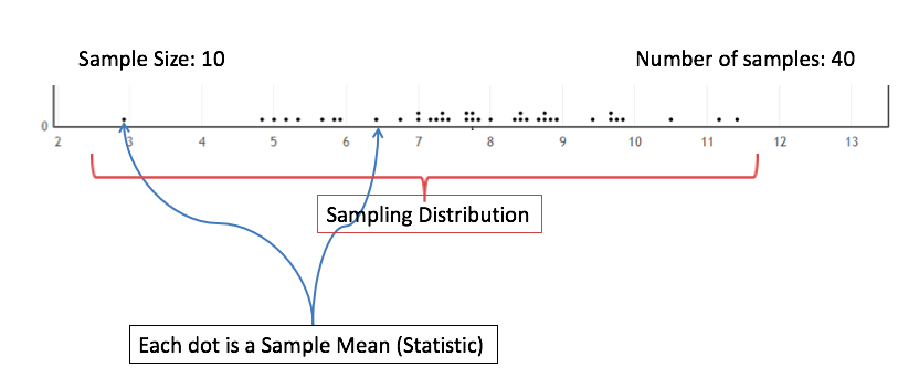
Sampling Distribution: The sampling distribution is the distribution of a statistic constructed by repeatedly sampling from the same population using the same sample size.

The next figure shows a simulated sampling distribution for the sample mean. Each of the 40 dots represents a sample mean from a sample of 10 individuals and together these statistics form the sampling distribution. We are interested in the properties of this distribution, in particular the shape, center, and spread of the statistics. To get a better idea of these qualities of the sampling distribution, we would need to sample many more statistics.

(A) The distribution of the sample.
This answer is not specific enough, what exactly do we collect from each sample?
(B) The distribution of population parameter.
The parameter is one fixed value and doesn't vary. Talking about the distribution of a parameter is therefore pointless.
(C) The distribution of the sample statistic.

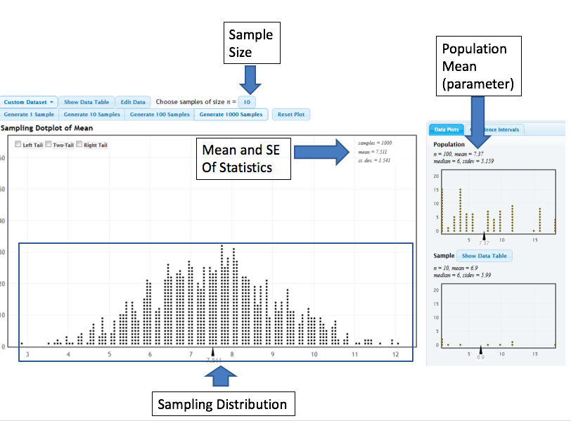
We have seen examples of a sampling distribution earlier in many of the activities so far in the course. We will use the StatKey Website to explore the sampling distribution of the sample mean. The image below illustrates the various components of the StatKey’s Sampling Distribution for a Mean page.

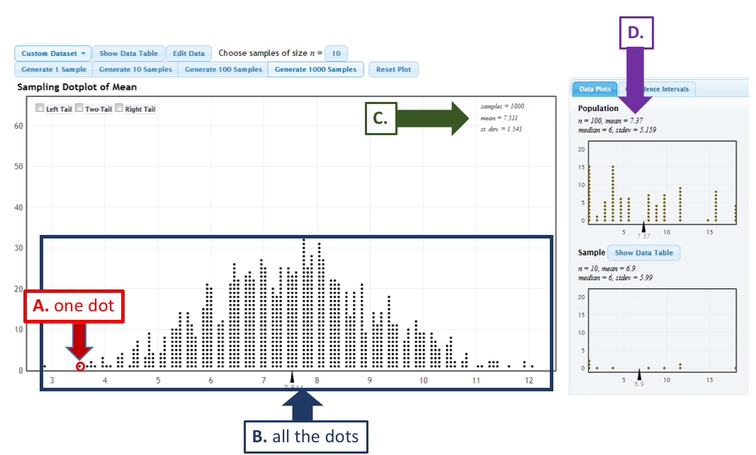
Check your Understanding

The following graph uses capital letters to label various elements of the StatKey sampling distribution page. Use these designations to answer each of the following questions.

(A) A
(B) B
(C) C
(D) D

(A) A
(B) B
(C) C
(D) D

(A) A
(B) B
(C) C
(D) D

(A) A
(B) B
(C) C
(D) D

3.4. The Central Limit Theorem¶

Note that a statistician would not necessarily carry out a simulation study such as this to answer a research question. Instead, one could use “short-cuts” known as a t-test or confidence interval to investigate a research question concerning a single population mean. These short-cuts are results of something known as the central limit theorem, which states the following:

The Central Limit Theorem for the Mean

Consider a random sample of n observations from ANY population with mean µ and standard deviation σ. The distribution of sample means will have a mean of \(\mu\) and a standard deviation of \(\sigma/\sqrt{n}\). When \(n\) (the number of subjects in the sample) is sufficiently large, this distribution will be approximately NORMAL; moreover, this approximation gets better as the sample size (\(n\)) increases.

We can see the Central Limit Theorem applied to the sample means calculated from our hypothetical population from Example 5.2 as follows:

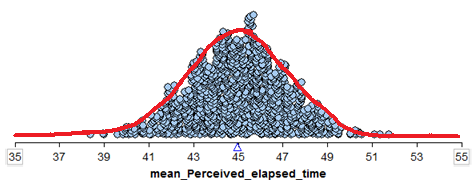
We see that this normal distribution is centered at the true population mean, \(\mu = 45\).
The standard deviation of all observations in our hypothetical population is \(\sigma = 9.4\) seconds. According to the central limit theorem, then, the standard deviation of the distribution of sample means is given by \(\sigma/\sqrt{n} = 9.4/\sqrt{20}=2.1\)
We see that the distribution of sample means is approximately normal.

Finally, recall from the previous chapter that given the mean and standard deviation of a distribution, we can determine whether a given observation is an outlier or not based on its position on this distribution. This will help us decide whether the sample mean actually observed in the research study is an outlier based on the distribution that assumes the null hypothesis is true.

The only question that remains is this: How large does n (the number of subjects in a study) have to be in order for us to use the short-cut provided by the Central Limit Theorem?

3.4.1. How large does n have to be?¶

We have seen that the distribution of the sample mean will not always be bell-shaped and often retains some of the features of the original population, such as a skewed shape. Next, we give some guidance on when it is reasonable to assume that the distribution of sample means will be normal.

Normal Population

If the original population is normally distributed, then the sampling distribution of the mean will also be normally distributed even if the sample size n is very small

(verify this using Tinkerplots as shown in class).

Skewed Population

The more skewed the distribution, the larger the sample size must be before the normal approximation fits the distribution of sample means well.

General Rule

For almost all populations, samples of size n ≥ 30 or 40 subjects will be sufficient to say that the distribution of sample means is approximately normal. However, if the distribution is very skewed, the sample size may have to be much larger than 30 in order for the central limit theorem to apply.

In summary, we can use the Central Limit Theorem to help us create procedures for answering questions about the population mean, be it comparing the mean to some hypothesized value or estimating the value of the population mean with an interval.

This works because:

We know the distribution of sample means will be approximately normal if either (i) the original population is normally distributed, or (ii) our sample size is sufficiently large.
We know the distribution of sample means will be centered at the true population mean

We know that the variability in the distribution of sample means is given by \(\sigma/\sqrt{n}\) (i.e., the variability decreases as the sample size gets larger, which we can see in the above examples).

In the next section, we put all of the pieces together to create what is a t-confidence interval. .. known as the t-test.

3.5. Assessing the Normality of a Data Set¶

The application of the central limit theorem (CLT) for means highlights the need for determining if a given data set is “normal.” In particular, we need to be careful about the application of the CLT to a small data set and a normal quantile plot will give us the needed tool.

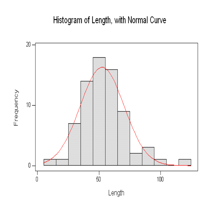
A first attempt at trying to determine that a data set is normal might involve drawing a normal curve over a dot plot or histogram. Unfortunately, it is difficult to determine how close a given histogram is to the curve.

A better solution is to use a normal quantile plot. These plots are designed to provide a simple distinction between data that is fairly normal and data that is not.

3.5.1. Creating a Normal Quantile Plot in JMP¶

The following GIF illustrates the process for constructing a normal quantile plot in JMP.

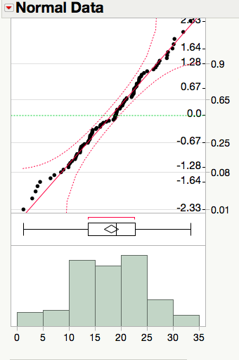
Reading a Normal Quantile Plot

Normal data is straight

A quantile plot with points that are close to a straight line indicate data that is fairly normal.

Non-normal data is curved

The presence of curvature in a quantile plot is an indication of the presence of tails that are longer or shorter than expected for data that comes from the normal distribution.

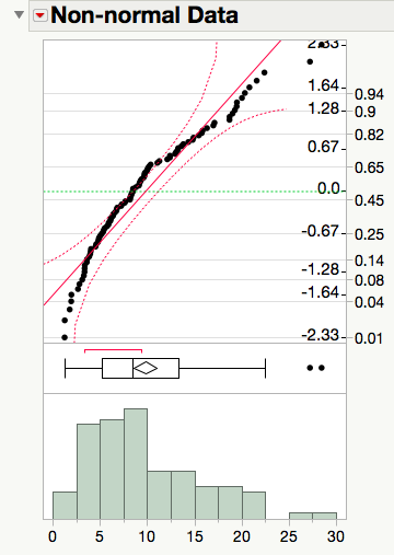As a consequence of the random nature of data, we need to allow for some flexibility in our interpretations of such graphs. Notice that each probability plot shown above includes curved confidence bands. These bands aid by giving us a visual cue about how picky we should be when determining the normality of a plot, only claiming the data is clearly non-normal when at least 5% of the points fall outside the bands.

(A) points with obvious curvature with a number of points outside the confidence bands.
(B) points that roughly form a straight line with almost all points falling inside the confidence bands.

(A) points with obvious curvature with a number of points outside the confidence bands.
(B) points that roughly form a straight line with almost all points falling inside the confidence bands.