4. Introduction to Confidence Intervals¶

In this chapter we will introduce some important ideas from statistics. We will be focusing on quantitative data and in particular estimation of a population parameter.

4.1. Confidence Intervals Basics¶

Recall that statistical inference is the process of using sample statistics to make guesses/inferences about a population parameter. One of the primary examples of this type of inference is estimating the value of a parameter.

In this section, we discuss the two types of estimates we can make (point and interval estimates), explore the proportion of sample means in a sampling distribution that fall within 2 standard errors of the mean, leverage this proportion to develop a good margin of error for a sample mean, put this all together to construct a confidence interval for the mean, and investigate what a statistician means when claiming to be “95% confident.”

Note

The other standard type of statistical inference involves testing a hypothesis about a parameter, a topic that we will devote more time on later in the course.

4.1.1. Point Estimates and Interval Estimates for Parameters¶

When estimating the value of a parameter, we can choose between one of two types of estimates.

Point Estimate: A point estimate is a single values estimate of the parameter (i.e. one number). Examples of point estimates are sample statistics like the sample mean and sample standard deviation that are used as point estimates for the population mean and population standard deviation, respectively.
Interval Estimate: An interval estimate consists of a range of values that we believe are likely to contain the actual parameter. Interval estimates usually come with a measure of how confident we are in the estimate (e.g. 95% confident).

When possible, it is best to use an interval estimate, because

We get a measurement of accuracy, as in how often the interval will successfully contain the parameter. This is called the confidence level of the interval. An interval that comes with a confidence level is called a confidence interval.
We get a sense of the precision of the estimate, which can be seen in the width of the interval. Specifically, more precise estimates have narrower confidence intervals.

(A) Point Estimate
(B) Interval Estimate

(A) Point Estimate
(B) Interval Estimate

4.1.2. Approximating the Standard Error of a Statistic¶

When constructing a confidence interval for the population mean, we will construct the interval by creating a buffer around the sample mean. To create this buffer, we add and subtract the margin of error to/from the sample mean. The right width of buffer is dependent on how spread out the sample means tend to be, i.e. the spread of the sampling distribution. The specific measure of spread that we use is the estimated standard deviation of the sample means, which is referred to as the standard error of the mean.

Margin of Error: The margin of error is the buffer that is added to and subtracted from the sample mean to construct an interval with a good chance of containing the population mean.
Standard Error of the Mean: Our estimate of the standard deviation of all sample means, taken from random samples of the same size, is called the standard error of the mean and demoted with SE.

(A) the amount of buffer that is added to and subtracted from the sample mean.
(B) a common mistake made by students in a statistics class when calculating the mean.
(C) the estimated standard deviation of the distribution of sample means.

4.1.3. Plus or Minus Two Standard Error and the Middle 95% of Statistics¶

For simplicity, we will focus on constructing a 95% confidence interval. It turns out that when the distribution of a statistic is symmetric and bell-shaped, going out 2 SE from the population mean will cover about 95% of the sample means.

To illustrate this fact, we have simulated the distribution of the sample mean using the StatKey Website, which is depicted in the figure shown below. The middle 95% of the sample means are shown with black dots, and we have colored the largest and smallest 2.5% of the sample means red. Furthermore, we can use this distribution to estimate the SE of the mean, which can be found in the top right of the graph. Notice that adding and subtracting 2 SE to the population mean leads to upper and lower bounds that are very close to the cut offs for the middle 95% of the distribution.

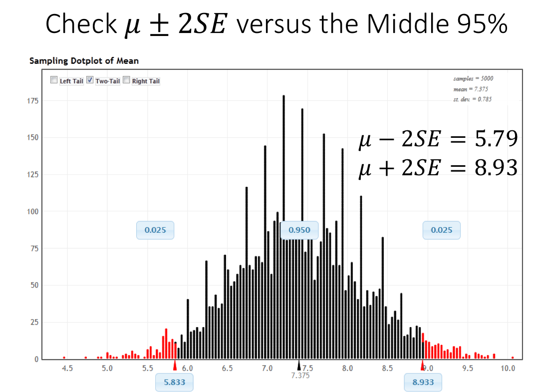
In the above figure we see that the limits generated by adding and subtracting 2 standard errors from the population mean (5.79 and 8.93) are very close to the cut-offs of the middle 95% of the distribution (5.83 and 8.93).

Caution

The above result will only work for distributions that are symmetric and bell shaped. We will need a different approach for skewed distributions.

Due to the fact that about 95% of the sample means are within 2 standard errors of the population mean, it makes sense to use this distance as the margin of error for a 95% confidence interval.

The Margin of Error for a 95% Confidence Interval for the Mean

The margin of error for a 95% confidence interval is given by

\[MoE = 2*SE\]

This margin of error works because

“A sample mean is in the middle 95% of the sample means” implies that the population mean will be within 2 SE of the sample mean.
Only the sample means in the lowest and highest 2.5% of the distribution will fail to capture the population mean in an interval using this margin of error.

In other words, if the sample mean is close enough to the population mean, the population mean is close enough to the sample mean.

The Main Point

If the sample mean is close enough to the population mean, the population mean is close enough to the sample mean. Using a margin of error of 2 standard errors means that about 95% of sample means are close enough.

Q-919: The interval constructed by adding and subtracting 2 SE to/from the: population mean will contain X% of the sample means. Identify the value of X.

(A) 100%
You are too *confident* (that is a statistics joke)
(B) 95%
(C) We can't determine X, as the samples were randomly selected.
While random samples are uncertain in the short term, they are predicitable in the long run.

4.1.4. Being (95%) Confident¶

Let’s make sure we are clear on what it means to be 95% confident. Consider the following figure, created using StatKey Website. Each of the dots is a sample mean and each of the line segments extends out 2 standard errors. The population mean is located at the solid vertical line, recall that our goal in constructing such an interval is to capture the population mean.

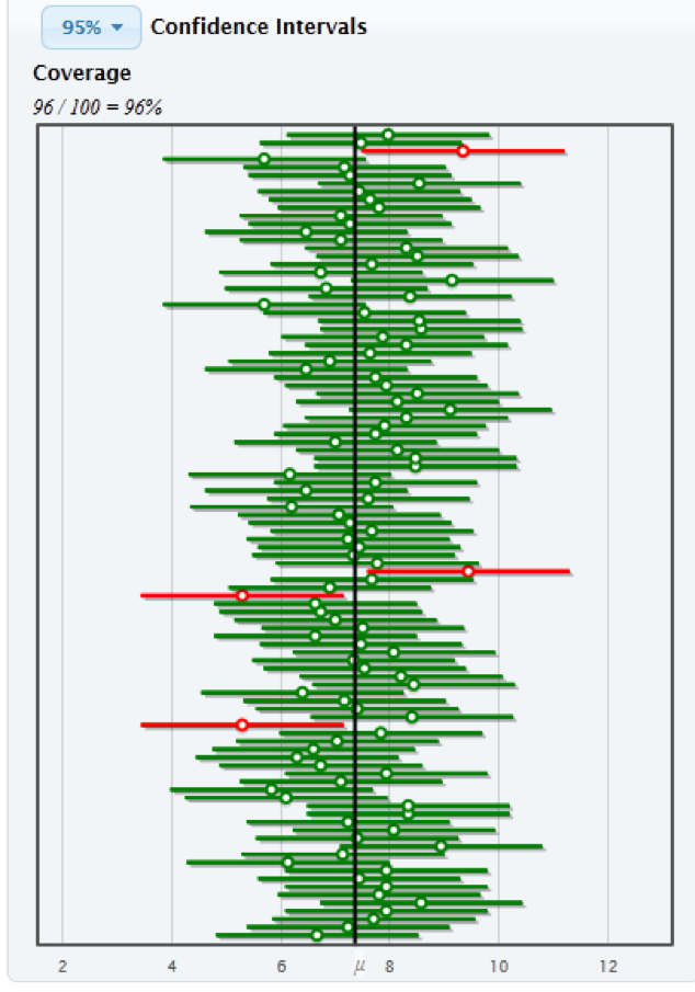
The intervals that are green successfully captured the population mean, and the intervals that failed to capture the population mean are colored red. Notice that about 95% of the intervals successfully capture the population mean.

Being “95% confident”

When a statistician says that she is “95% confident”, she means that she is using a procedure, that when used repeatedly on many random samples, will work 95% of the time.

Caution

We purposely avoid the phrase “95% probability”. This is because each specific interval either works 100% of the time (captured the mean) or fails 100% of the time (fails to capture the mean). For example, suppose we take a sample and construct an interval, which turns out to be from 2.4 to 7.6. The population mean is either between these numbers or it is not. Using “95% probability” in place of “95% confidence” makes it sound like this specific interval only works some of the time, when in fact it either always works or never works.

(A) We are really pretty sure of the result.
This answer is too vague, try being more specific.
(B) The interval we constructed from a specific sample will work 95% of the time.
Unfortunately, any single interval either works 100% of the time or 0% of the time.
(C) We are using a procedure that works 95% of the time, when applied to many, many samples.
Statisticians define success "in the long run."

4.2. Bootstrap Confidence Intervals¶

Our current method for finding a confidence interval involves the following steps:

Simulate the sampling distribution of the mean by taking many samples from the population.
Compute the standard error, i.e. the standard deviation of the statistics in the simulated distribution.
Add and subtract 2 times this value to get a 95% confidence interval.

Unfortunately, there is a big problem with this approach.

Caution

Problem with the Current Approach

We need to know the whole population to produce the standard error. This approach is very impractical, as taking a census is either very expensive and many times impossible.

Our solution will be to use a bootstrap sample, which is acquired by sampling the sample.

4.2.1. Bootstrap Samples¶

Since we can’t be expected to have the entire population at our disposal, we will use the best tool at our disposal: the sample. Instead of taking many samples from the population to simulate the sampling distribution, we will take many bootstrap samples from the sample, allowing us to simulate the bootstrap distribution.

Bootstrap Samples

A bootstrap sample is a sample of the sample that uses

Sampling with replacement.
The same sample size as the original sample.

Bootstrap Statistic

A bootstrap statistic is a statistic taken from a bootstrap sample.

Bootstrap Distribution

The bootstrap distribution is the distribution of many, many bootstrap statistics.

Bootstrap Standard Error

The bootstrap standard error is the standard deviation of bootstrap distribution, which can be used as an estimate of the actual standard error of a statistic.

Using sampling with replacement allows for some variability from one bootstrap sample to the next, as some values will be selected more than once and other values will be left out of the sample. It turns out that the variability between bootstrap statistics is very similar to the variability between the actual statistics in the sampling distribution.

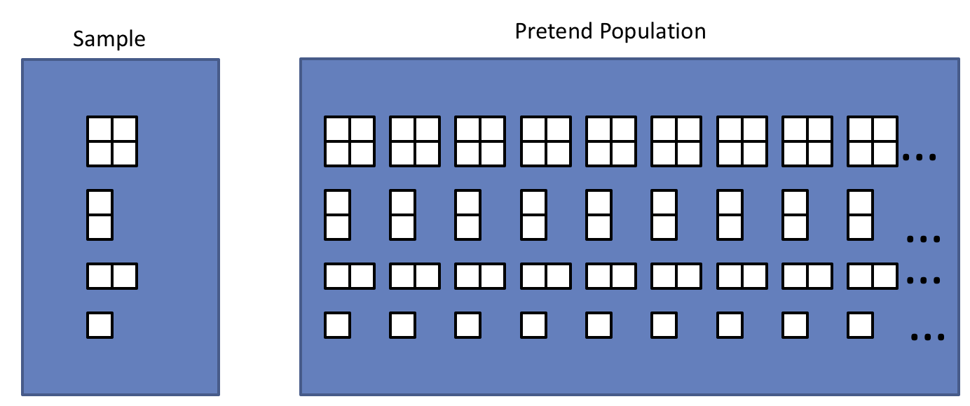
Another way to understand bootstrap samples is to imagine that we are sampling from a population where we have huge stacks of copies of each item in the sample. In effect we are using the best approximation for the population that we have available.

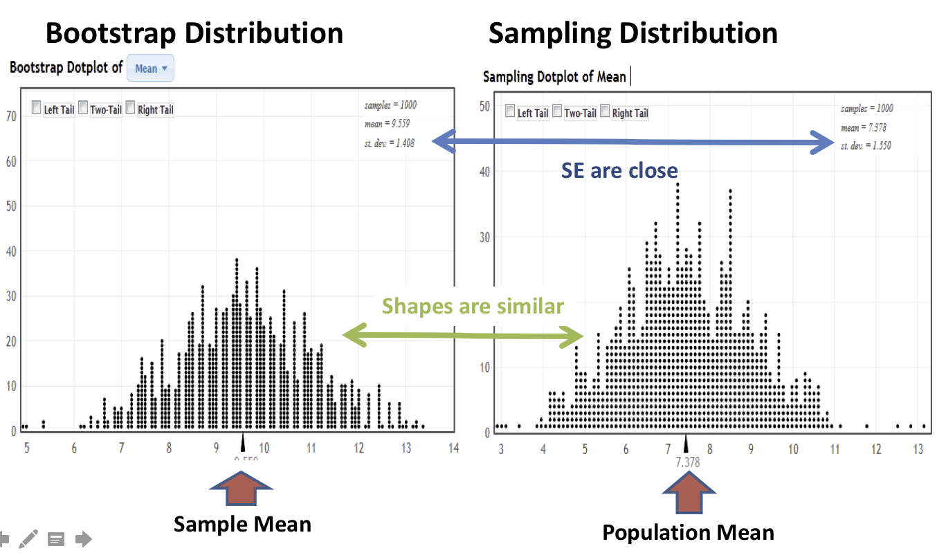
In the next image, we illustrate the process of constructing the bootstrap distribution using the StatKey’s Confidence Intervals for a Mean page. The bootstrap distribution is constructed by repeating steps 1-3 many times.

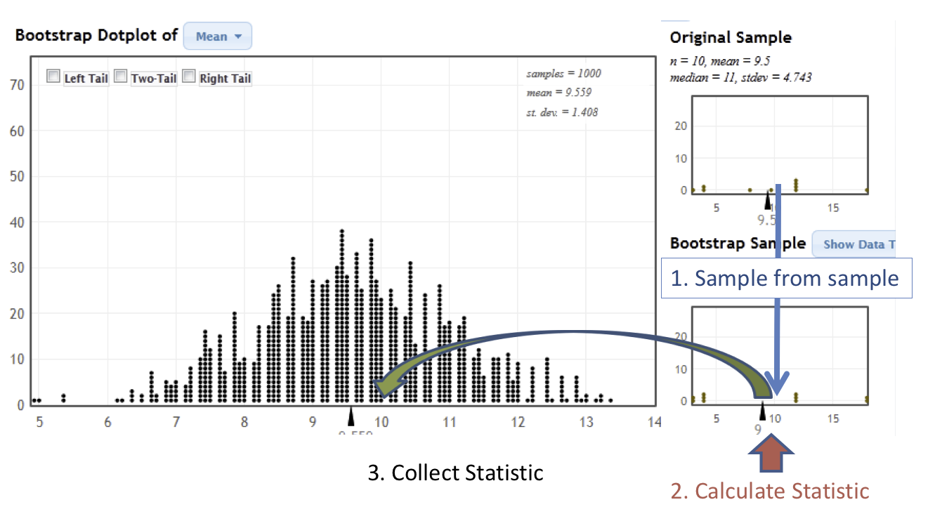
Finally, we will compare and contrast the sampling distribution and the bootstrap distribution. The two distributions tend to have the same shape and spread, but different centers. In particular, the sampling distribution is centered at the population mean and the bootstrap distribution is centered at the original sample mean.

(A) a sample of the sample.
(B) a statistic from a sample of a sample.
(C) a collection of statistics from a sample of a sample.
(D) the standard deviation of statistics from a sample of a sample.

(A) a sample of the sample.
(B) a statistic from a sample of a sample.
(C) a collection of statistics from a sample of a sample.
(D) the standard deviation of statistics from a sample of a sample.

(A) a sample of the sample.
(B) a statistic from a sample of a sample.
(C) a collection of statistics from a sample of a sample.
(D) the standard deviation of statistics from a sample of a sample.

(A) a sample of the sample.
(B) a statistic from a sample of a sample.
(C) a collection of statistics from a sample of a sample.
(D) the standard deviation of statistics from a sample of a sample.

4.2.2. Constructing Bootstrap Confidence Intervals¶

Now we have two choices for making a confidence interval using the bootstrap distribution.

Use the bootstrap standard error to construct a 95% confidence interval by adding and subtracting a margin of error of \(2SE\).
Use the limits of the middle 95% of the bootstrap statistics as the boundaries for our 95% confidence interval.

The advantage of the second approach is that we can quickly and easily change the level of confidence of the interval by changing the middle percentage. For example, if we want a 99% confidence interval, we will highlight the middle 99% of the bootstrap statistics and use the lower and upper bounds of this collection for our confidence interval.

On the other hand, if we wanted to construct a confidence interval using the bootstrap standard error for a confidence level that is different than 95%, we would need to figure out how many standard errors to use for the margin of error. There is a theoretical solution to this problem, which we will highlight in the next section.

4.3. Confidence Intervals Based on the Normal Distribution¶

In our bootstrap activities we have seen some common results.

Important Points

The distribution of the sample mean was often (but not always) a bell-shaped curve.
Using a margin of error of 2 standard errors resulted in intervals that worked about 95% of the time.

In this section, we leverage these facts and introduce a theoretical approach to confidence intervals that will save us the work of running a simulation every time we want an interval.

4.3.1. Example 5.1:¶

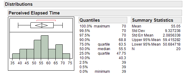
A study conducted by researchers at Pennsylvania State University investigated whether time perception, a simple indication of a person’s ability to concentrate, is impaired during nicotine withdrawal. The study results were presented in the paper “Smoking Abstinence Impairs Time Estimation Accuracy in Cigarette Smokers” (Psychopharmacology Bulletin [2003]: 90-95). After a 24-hour smoking abstinence, 20 smokers were asked to estimate how much time had passed during a 45-second period. Suppose the resulting data on perceived elapsed time (in seconds) were analyzed as shown below (these results are artificial but are similar to the actual findings). The data can be found in the file Nicotine1.JMP.

We can use JMP to summarize the data as follows:

(A) 55.05
That is the mean of the data.
(B) 9.33
That is the standard deviation of the data.
(C) 2.09
That is the standard error of the mean.

(A) 55.05
That is the mean of the data.
(B) 9.33
That is the standard deviation of the data.
(C) 2.09
That is the standard error of the mean.

(A) Yes
We would expect some variability from one sample to the next.
(B) No
We would expect some variability from one sample to the next.

4.3.2. Example 5.2: Another “simulation study”….¶

Suppose we set up a hypothetical population of smokers suffering from nicotine withdrawal, which was created using bootstrap samples from the original sample. This population has been purposefully created so that the mean perceived elapsed time is exactly 45 seconds.

Note that in reality, the true population mean is usually an unknown quantity which we are trying to estimate. Since it is not feasible to collect data on the entire population of smokers suffering from nicotine withdrawal, the researchers took a random sample of 20 subjects in order to estimate the average perceived elapsed time. We will illustrate how to take bootstrap samples from this sample using Tinkerplots.

Note

We could have also used the StatKey website to simulate this distribution, but we use this example as a chance to introduce Tinkerplot’s functionality.

4.3.3. Simulating the Bootstrap Distribution in Tinkerplots (Optional)¶

Each of the elements in the mixer represents the perceived elapsed time for a smoker suffering from nicotine withdrawal in the population (e.g., the highlighted subject thought that 50 seconds had passed during a 45-second period). We set the repeat value to 20 in order to randomly select 20 subjects from the population for our study.

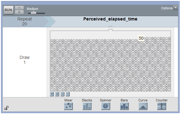
Click Run to randomly select our first sample of 20 subjects, and we can then create a plot of their perceived elapsed times. Note that the mean of these 20 subjects is shown on this plot.

4.3.4. Sample # 1:¶

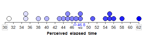
Questions:

What is the average (or mean) perceived elapsed time of the 20 subjects in this study?
Does this necessarily mean that the average perceived elapsed time is greater than 45 seconds for all smokers suffering from nicotine withdrawal? What would you say to a researcher who tried to use only this sample mean to draw this conclusion?

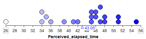
Even though in reality we would carry out a study only once, we will use Tinkerplots to take a sample of 20 subjects from this population over and over again so that we get an idea of how much the sample mean could change from sample to sample. Our second and third random samples of 20 subjects and their sample means are shown below:

4.3.5. Sample #2:¶

4.3.6. Sample #3:¶

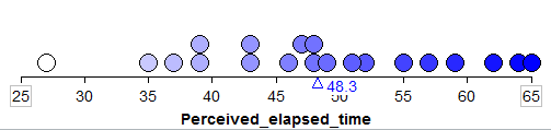
We can start to collect these sample means in a new plot to create the distribution of sample means:

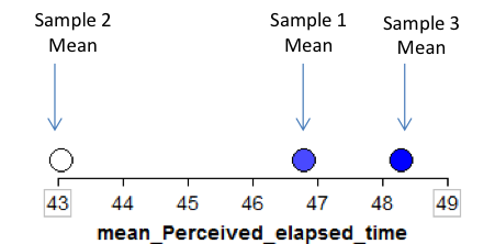
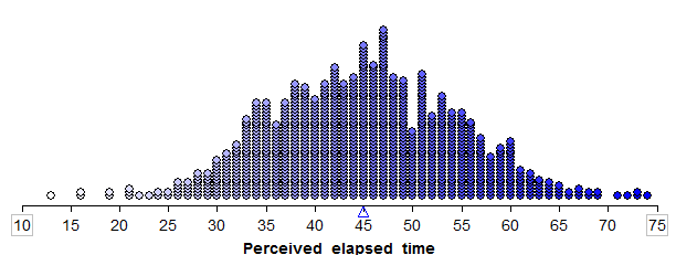
To get a really good idea of what values are likely to occur by chance when taking random samples of size 20 from the population, we should take more than just three samples. The graphic below shows the process we used to create the distribution of sample means and the final plot of the means of 1,000 random samples.

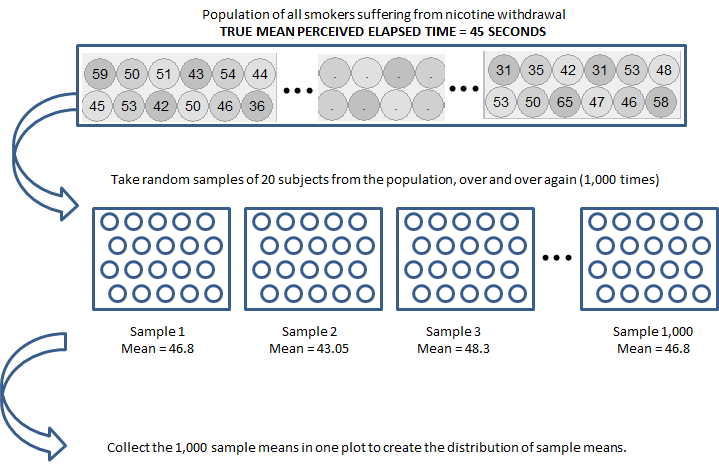
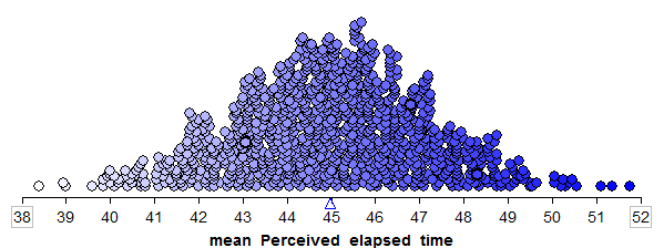
This is a distribution of sample means. Recall that these 1,000 samples (each consisting of 20 subjects) came from a population with a true mean perceived elapsed time of 45 seconds. So, this distribution gives us a good idea of what sample means from 20 subjects are likely (or unlikely) to occur by chance if the true mean is 45 seconds.

4.3.7. Confidence Interval for a Single Population Mean¶

In Example 5.1, we found evidence that the mean perceived elapsed time for smokers suffering from nicotine withdrawal significantly differed from the actual 45 seconds of time that had elapsed. Our next question is obvious: HOW MUCH does it differ? To answer this question, we must construct a confidence interval.

Recall our discussion of confidence intervals from earlier in the semester:

This procedure does NOT require any hypotheses concerning our population parameter of interest (the mean, in this case). We will use both our sample data (in particular, the observed mean) and what we know about the distribution of sample means to obtain a range of likely values for our population mean.

Comments

A confidence interval allows us to estimate the population parameter

of interest (recall that the hypothesis test does NOT allow us to do this). Therefore, when available, a confidence interval should always accompany the hypothesis test.
The confidence interval does not require any hypothesized value for

the population parameter. Instead, we center the confidence interval on the sample mean. Consider the following example.

Example 5.4: Our goal is to construct a 95% confidence interval for the mean perceived elapsed time for smokers suffering from nicotine withdrawal. To do this, we will center our distribution of sample means on the observed mean. Then, we will find the lower and upper endpoints that separate the middle 95% of the distribution from the rest (since we are constructing a 95% confidence interval).

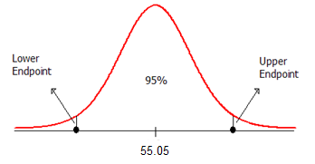
The formula for calculating the endpoints of this confidence interval is given as follows:

\[\bar{x} \pm t_{quantile}\frac{s}{\sqrt{n}}\]

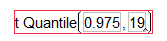
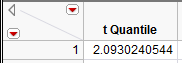
The appropriate t-quantile can be found using JMP. To find this value, you need the following information:

confidence level =
df =

Open a new JMP data table and choose Probability > t Quantile from the Formula editor. Enter the following:

Here is an animated GIF of the process.

For this example, JMP returns the following t-quantile:

Also, recall from Example 5.1 that the mean and standard deviation are as follows:

Use this information to find the endpoints of the confidence interval:

Lower endpoint: \(\bar{x}-t_{quantile}\left(s/\sqrt{n}\right) = 55.05 - 2.093*\frac{9.327}{\sqrt{20}} = 50.68\)

Upper endpoint: \(\bar{x}+t_{quantile}\left(s/\sqrt{n}\right) = 55.05 + 2.093*\frac{9.327}{\sqrt{20}} = 59.42\)

4.3.8. Confidence Intervals for the Mean in JMP¶

Note that JMP automatically provides the endpoints of the 95% confidence interval for this mean when you analyze the distribution of the variable of interest.

Questions:

Interpret the meaning of this interval. What does this interval tell us about the true mean perceived elapsed time for all smokers that are suffering from nicotine withdrawal?
Does this interval agree with what you learned from the hypothesis test? Explain.
How would your calculations change if you wanted to obtain a 90% confidence interval, instead?

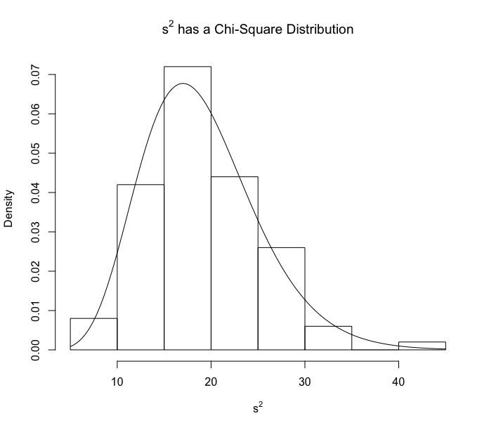
4.3.9. Confidence Intervals for the Population Standard Deviation¶

If the original population is bell-shaped, then there is also a formula for the population standard deviation. This is due to the fact that, for normal data, the distribution of the standard deviation squared (also known as the variance) has a chi-square distribution.

While it is certainly possible to compute a confidence interval using the formula, it is more convenient to compute these intervals using the built-in JMP functions. We can generate a confidence interval for both the population mean and standard deviation as follows.

Constructing Confidence Intervals for the Mean and Standard Deviation in JMP

Enter the sample data in a new data table.
Perform ANALYZE > DISTRIBUTION on the column of interest.
Click on the triangle above the distribution and select confidence intervals.

Caution

We need to make sure that the original data is fairly normal before relying on the formula for the confidence interval for a standard deviation. If there is any doubt about this normality, we would be better off using the bootstrap interval instead.

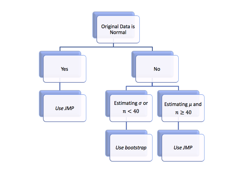
4.4. Picking the Correct Procedure¶

Now that we have a choice between using the bootstrap and using the JMP intervals, we need some rules on which procedure is the right procedure for a given data set. The advantage of JMP is the ease of use, but the JMP procedures require normality in some form (either normality of the original data or normality through a large sample in the case of estimating \(\mu\)).

Using JMP is viable when

Estimating \(\mu\):
Using JMP to construct a confidence interval for \(\mu\) is viable when
1. The original data is normal, or
2. The sample size is large (\(n \ge 40\))
Estimating \(\sigma\):

Using JMP to construct a confidence interval for \(\sigma\) is viable when the original data is normal.

Luckily, the bootstrap confidence intervals don’t require any assumptions about normality and can be used when the JMP intervals are not viable. The following flow chart illustrates the decision process involved in deciding which procedure is correct for a given data set.

Recall that we use a normal probability plot to decide if the original data is normal. Consequently, we will perform the following steps when constructing a confidence interval.

Main Steps in Constructing a Confidence Interval for \(\mu\) or \(\sigma\)

Use JMP to construct a normal quantile plot and check the normality of the original data.
Determine the correct procedure based on normality and the sample size.
Construct your confidence interval.
Write a sentence summarizing your interval in the context of the problem.

(A) JMP interval
Since the original data is normal, it is safe to use JMP.
(B) Bootstrap interval
Since the original data is normal, it is safe to use JMP. We might as well pick the procedure that requires less work.

(A) JMP interval
Since the original data is normal, it is safe to use JMP.
(B) Bootstrap interval
Since the original data is normal, it is safe to use JMP. We might as well pick the procedure that requires less work.

(A) JMP interval
Since the original data is not normal and the sample size is small, it is safer to use the bootstrap intervals.
(B) Bootstrap interval
Since the original data is not normal and the sample size is small, it is safer to use the bootstrap intervals.

4.5. Confidence Intervals for Regression¶

Recall that statistical inference is the process of making guesses about population parameters using a random sample. We can apply the same ideas we used earlier in the book to linear regression, estimating the values of the population correlation coefficient and/or the slope of the population regression line. In this section, we will apply the bootstrap process to regression to obtain confidence intervals for these quantities.

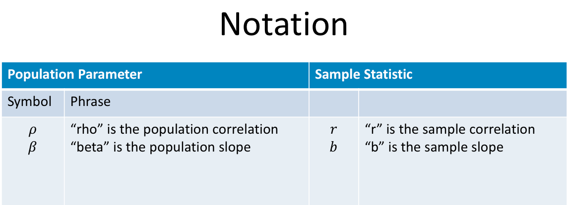
4.5.1. Notation for Regression¶

The following figure gives the common symbols used for the sample and population correlation coefficients and slopes. Once again, greek letters are used for the parameters, in this case \(\rho\) and \(\beta\) for the correlation coefficient and slope, respectively. The sample correlation coefficient and sample slope are respectively denoted by \(r\) and \(b\).

4.5.2. Bootstrap Intervals for Regression¶

Our goal is to use the sample values of \(r\) and \(b\) to estimate \(\rho\) and \(\beta\). We can again estimate the sampling variability in these statistics by using the bootstrap. Let’s review the process of generating the bootstrap distribution of a statistic.

Generating the bootstrap distribution of a statistic

Generate many samples of the sample (at least 1000) by taking samples that
1. use the same size as the original sample
2. use sampling with replacement
For each sample, compute the value of the bootstrap statistic.
Collect all of these bootstrap statistics into the bootstrap distribution. We can construct C% confidence intervals using the middle C% of this distribution.

Once again, we will use the StatKey Website, this time in the section titled Confidence Interval for a Slope, Correlation

Next Section - 5. Introduction to Hypothesis Tests