4.6. Levels of Abstraction
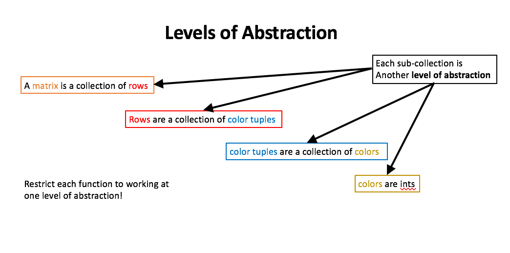
Good practice when working with lists, matrices and other arrays is keeping our functions restricted to one level of abstraction. For example, when working with an image we have four levels of abstraction, as illustrated below.
A clean and modular approach to writing functions and comprehensions involves restricting each function to one level of abstraction. We will illustrate this process by transforming an image to grayscale.
4.6.1. Example 1 - averaged grayscale image transformation
There are four levels of abstraction found in an RGB numpy array. These
consist of a matrix of rows (or columns), a row of RGB tuples, a RGB tuple of
colors and the colors themselves. Gray RGB tuples have the same number in all
three entries. There a number of ways to perform a grayscale transformation, one
of which is replacing each color with the average of the original colors.
In this example, we will use a bottom-up approach by starting with the lowest level of abstraction and working up one level at a time. At each new level, we will apply the function from the last level to each element in the next level.
Lowest Level - A color
Thinking in terms of levels of abstraction, we will start at the lowest level of abstraction and create a function that returns the average color of a color tuple. We need to be careful of overflow when working with finite precision integers and if we added all of the colors before dividing, there is a definite possibility of overflow. Consequently, we will multiple each color by 1/3 before adding.
In [1]: import numpy as np

In [2]: example_color = np.array([100, 200, 250], dtype = np.uint8)

In [3]: average_color = lambda tup: sum([c//3 for c in tup])

In [4]: color = average_color(example_color)

In [5]: color
Out[5]: 182
Level 2 - RGB tuple
The next level of abstraction is a RGB tuple. For this example, we need to
create a tuple that contains average_color three times and the range
function will be useful here.
In [6]: average_RGB_tuple = lambda tup: [average_color(tup) for i in range(3)]

In [7]: average_RGB_tuple(example_color)
Out[7]: [182, 182, 182]
Level 3 - Row of RGB tuples
Now we apply the average_RGB_tuple function to all tuples in a row.
In [8]: example_row = np.array([[100, 200, 250], [20, 0, 115]], dtype=np.uint8)

In [9]: averaged_row = lambda row: [average_RGB_tuple(tup) for tup in row]

In [10]: averaged_row(example_row)
Out[10]: [[182, 182, 182], [44, 44, 44]]
Level 4 - Matrix of rows
Finally, we apply the averaged_row to each of the rows in the matrix.
In [11]: example_matrix = np.array([example_row, example_row + 5], dtype=np.uint8)

In [12]: example_matrix
Out[12]:
array([[[100, 200, 250],
        [ 20,   0, 115]],

       [[105, 205, 255],
        [ 25,   5, 120]]], dtype=uint8)

In [13]: averaged_matrix = lambda mat: np.array([averaged_row(row) for row in mat])

In [14]: gray_pic = averaged_matrix(example_matrix)

In [15]: gray_pic
Out[15]:
array([[[182, 182, 182],
        [ 44,  44,  44]],

       [[188, 188, 188],
        [ 49,  49,  49]]])
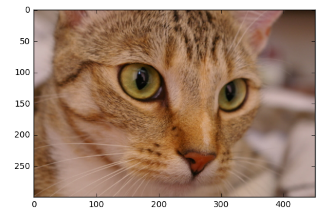
In closing, we will apply this transformation to our good friend Chelsea the cat.
import matplotlib.pylab as plt
%matplotlib inline
from skimage import data
cat = data.chelsea()
plt.imshow(cat)
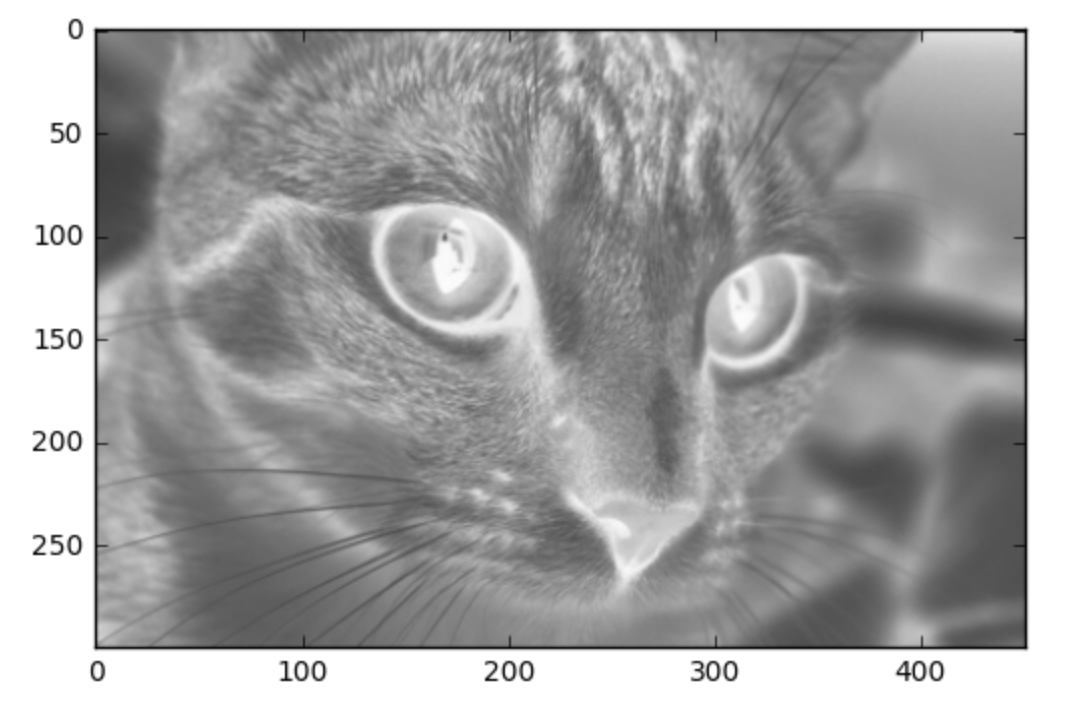
Here is Chelsea after applying the averaged grayscale transformation.
averaged_cat = averaged_matrix(cat)
plt.imshow(averaged_cat)
4.6.2. Example 2 - lightness grayscale transformation
In the last example, we used a bottom-up approach to designing our program. In this next example, we will instead use a top-down approach by starting with the highest abstraction level and work our way down. Using a top-down approach is considered a good practice, but it will seem strange at first because we will need to call functions that we haven’t designed yet. In fact, when using the top-down approach, we will discover what functions need to be written as we go.
Top Level - Matrix of rows
We start by writing a function that will apply the lightness transformation to
each row. To do this, we need a (as yet defined) function that will be applied
to each row. Let’s call it lightened_row. This function will take a row
and return a row that contains transformed tuples.
In [16]: lightened_matrix = lambda mat: np.array([lightened_row(row) for row in mat], dtype = np.uint8)
See! We just invented the purpose of the next function without even trying.
Level 3 - Rows of tuples
Now we need to write the lightened_row function. This function will apply
the lightness transformation to each of the tuples in the row. To do this we
need a function that will perform this transformation on a tuple. Call it
lightened_tuple. Don’t worry about how it will work, we will get to that in
a bit.
In [17]: lightened_row = lambda mat: [lightened_tuple(tup) for tup in row]
Isn’t using non-existent function freeing! Time to move down another level.
Level 2 - Tuple of colors
Time to create the lightened_tuple function. This function will need to
return a tuple of three colors, each of which will be the same value. We will
need a function that will compute the lightness color for a given tuple. Call
it lightness. (You guessed, we will wait to define it until we get to the
next layer of abstraction.)
In [18]: lightened_tuple = lambda tup: [lightness(tup) for i in range(3)]
Level 1 - Compute the lightness color
Finally, we can define the last function (and stop living in make-believe land).
The lightness transformation involves replacing all three colors in a tuple with
the average of the max and min colors. As before, we need to be careful
to avoid overflow, which will be accomplished by dividing then adding.
In [19]: lightness = lambda tup: max(tup)//2 + min(tup)//2
Consider giving the top-down approach a try sometime!
Note
You will apply a third grayscale transformation in the exercises found at the end of the chapter.