7.6. Common Patterns for Processing Sequences with Dictionaries¶

In this section, we will illustrate a number of common patterns for processing lists using dictionaries. These patterns include counting frequencies, counting frequencies by some key function and grouping data by some key or key function. In each case, we will start by looking at the imperative solution, then move on to building a high-level abstraction and finally use a pre-existing function from toolz.

7.6.1. Maps and filters for dictionaries¶

The toolz module contains maps and filters for dictionary keys, values, and items. In the same way that we can chain map, filter and reduce together to solve most list processing problems; keymap, keyfilter, valmap, valfilter, itemfilter and itemmap can be useful when processing dictionaries. We will illustrate with by redoing two exercises from an earlier homework.

7.6.1.1. Example 1 - average quiz scores¶

To see these tools in action, let’s revisit a homework exercise from a previous chapter (Chapter 5 Exercise 2). In this example, we have a number of quiz scores stored in a file. Each line of the file contains the students name followed by each quiz score.

We start by splitting the lines.

In [1]: file_str = '''joe 10 15 20 30 40
   ...: bill 23 16 19 22
   ...: sue 8 22 17 14 32 17 24 21 2 9 11 17
   ...: grace 12 28 21 45 26 10
   ...: john 14 32 25 16 89'''
   ...: 

In [2]: lines = file_str.split('\n')

In [3]: lines
Out[3]: 
['joe 10 15 20 30 40',
 'bill 23 16 19 22',
 'sue 8 22 17 14 32 17 24 21 2 9 11 17',
 'grace 12 28 21 45 26 10',
 'john 14 32 25 16 89']

Next we split each line into list of words. Earlier this would have been accomplished using a list comprehension as follows.

In [4]: words =  [line.split() for line in  lines]

In [5]: words
Out[5]: 
[['joe', '10', '15', '20', '30', '40'],
 ['bill', '23', '16', '19', '22'],
 ['sue', '8', '22', '17', '14', '32', '17', '24', '21', '2', '9', '11', '17'],
 ['grace', '12', '28', '21', '45', '26', '10'],
 ['john', '14', '32', '25', '16', '89']]

but now we recognize this as a map, and perform the same task using a map.

In [6]: words = list(map(lambda line: line.split(), lines))

In [7]: words
Out[7]: 
[['joe', '10', '15', '20', '30', '40'],
 ['bill', '23', '16', '19', '22'],
 ['sue', '8', '22', '17', '14', '32', '17', '24', '21', '2', '9', '11', '17'],
 ['grace', '12', '28', '21', '45', '26', '10'],
 ['john', '14', '32', '25', '16', '89']]

We start by forming a dictionary with key’s equal to the names (i.e. first of each row) and value containing all the rest of the line. Since the drop function is lazy, we will compose it with list to force completion for this small example.

In [8]: from toolz.curried import first, drop, compose

In [9]: rest = compose(list, drop(1))

In [10]: scores = {first(line):rest(line) for line in words}

In [11]: scores
Out[11]: 
{'bill': ['23', '16', '19', '22'],
 'grace': ['12', '28', '21', '45', '26', '10'],
 'joe': ['10', '15', '20', '30', '40'],
 'john': ['14', '32', '25', '16', '89'],
 'sue': ['8', '22', '17', '14', '32', '17', '24', '21', '2', '9', '11', '17']}

We wish to compute the average quiz score. Consider the levels of abstraction for this problem.

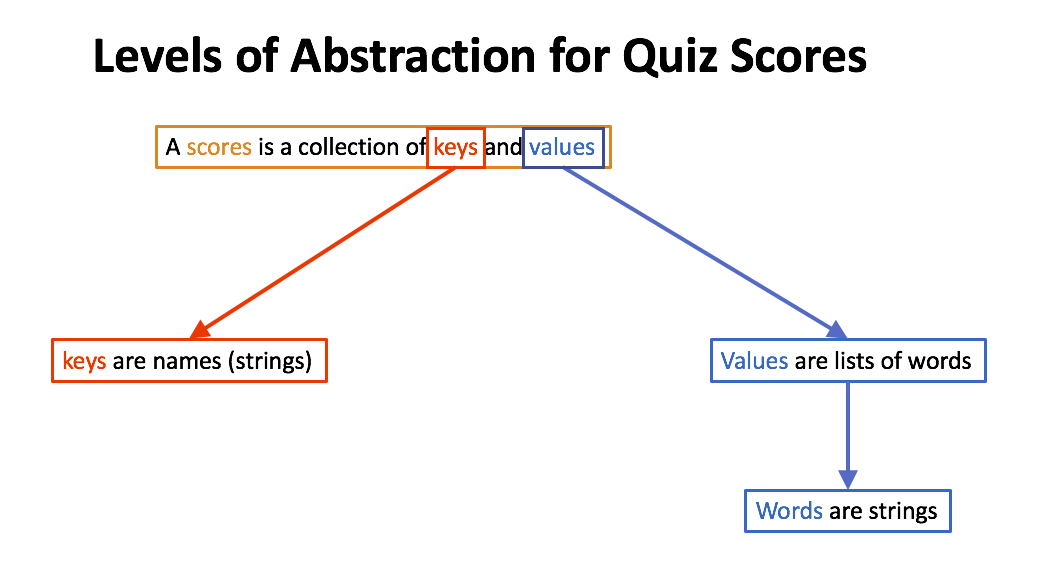
Levels of abstraction for the quiz score dictionary.

The score dictionary consists of keys (strings) and values (lists of words).

If we are to obey the clean code rules for writing and composing function, we should write functions at each level of abstraction, that is functions that

Level 1 Process score
Level 2 Process lists of scores
Level 3 Process a dictionary of name-list pairs

Level 1 Functions: What is it that we want to do to each word?

We need to turn them into integers, which is accomplished with int.

Level 2 Functions: What do we need to do to the list of words?

Turn each score into an integer. map(int)
Turn this lazy map into a list list
Compute the mean of the list of integers mean = lambda L: sum(L)/len(L)

Notice that each of the functions acts on a list, i.e. the right level of abstraction. We will combine these using composition, which is illustrated below.

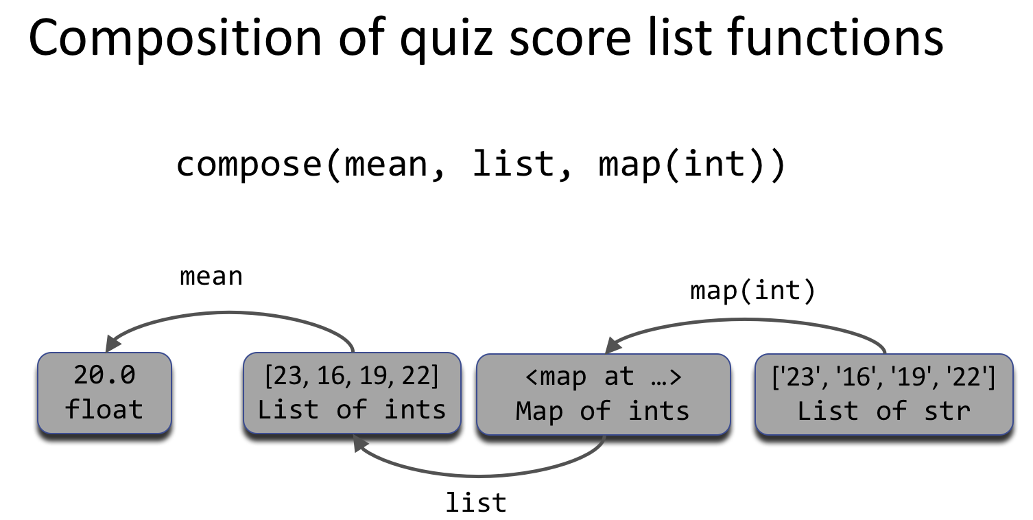
The composition of quiz score list functions.

To process each value (quiz score list), we apply compose(mean, list, map(int)). Recall that functional composition is applied from right to left, with map(int) first converting each string to an int, then list converts the lazy map to a list, and finally mean computes the average of the list.

Level 3 Functions: What do we want do to the keys/values for the dictionary?

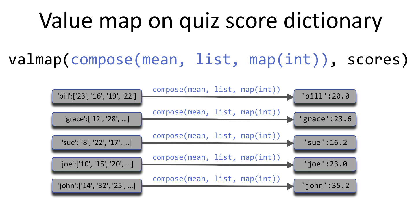
In this case, we need to apply the function from the last level of abstraction to each of the values in the dictionary.

To do this we do this using valmap, which applies a function to each value in the dictionary. There is no need to change the keys.

Using valmap to processes each value in the scores dictionary.

By applying valmap, we apply the function from the last level of abstraction to each of the values in the scores dictionary.

In [12]: from toolz import valmap

In [13]: from toolz.curried import map

In [14]: mean = lambda L: sum(L)/len(L)

In [15]: scores = valmap(compose(mean, list, map(int)), scores)

In [16]: scores
Out[16]: 
{'bill': 20.0,
 'grace': 23.666666666666668,
 'joe': 23.0,
 'john': 35.2,
 'sue': 16.166666666666668}

In this example, we show an important technique for applying maps. When we want to apply transformations in sequence, we use composition with a curried map. On the other hand, when we want to perform multiple maps sequentially, we compose the map helper functions to perform all transformations in one pass.

Note

Computing the mean of a lazy sequence is difficult as (a) sequences like map don’t have a length and (b) we can only process the sequence once before it is empty. We will revisit this topic when we go into more detail about lazy evaluation in Python in an upcoming section.

Let’s peel apart valmap(compose( mean, list, map(int)), scores) to make sure we can interpret composition of this type. We start by reinitializing the raw scores and applying each function in the compose(mean, list, map(int)) recall that the function inside of valmap is meant to act on each of the inner list values. For illustration, we will work on 'sue'.

In [17]: from toolz import get

In [18]: scores = {first(line):rest(line) for line in words}

In [19]: sue_scores = get('sue', scores)

In [20]: func = map(int)

In [21]: sue_scores = func(sue_scores)

In [22]: sue_scores
Out[22]: <map at 0x10a83fb38>

Remember that map(int) is the curried partial function that is equivalent to lambda L: map(int, L). Due to the lazy nature of map, and in particular the lack of a length, we apply the list conversion function.

In [23]: func = list

In [24]: sue_scores = func(sue_scores)

In [25]: sue_scores
Out[25]: [8, 22, 17, 14, 32, 17, 24, 21, 2, 9, 11, 17]

Now that the values are list of integers, we can compute the mean.

In [26]: func = mean

In [27]: sue_scores = func(sue_scores)

In [28]: sue_scores
Out[28]: 16.166666666666668

Of course these three function calls can be composed into one call. Remember that compose applies the functions from right to left.

In [29]: sue_scores = get('sue', scores)

In [30]: func = compose(mean, list, map(int))

In [31]: func(sue_scores)
Out[31]: 16.166666666666668

To apply this function to each of the values in our quiz score dictionary, we use valmap to map it to all of the values.

In [32]: func = compose(mean, list, map(int))

In [33]: valmap(func, scores)
Out[33]: 
{'bill': 20.0,
 'grace': 23.666666666666668,
 'joe': 23.0,
 'john': 35.2,
 'sue': 16.166666666666668}

While it is often advisable, there is no need to assign our helper function to a external variable. Using substitution, the final expression becomes

In [34]: valmap(compose(mean, list, map(int)), scores)
Out[34]: 
{'bill': 20.0,
 'grace': 23.666666666666668,
 'joe': 23.0,
 'john': 35.2,
 'sue': 16.166666666666668}

This example illustrates the proper application of functional constructs such as map, compose and valmap allows us to express complex computations in a succinct form. On the other hand, programmers should always be careful not to be too clever when expressing a computation, always keeping an eye out for readability. The reader that is new to functional programming might need to work at translating an expression like the one shown above, but it will become second nature after a while.

Advice on reading maps, pipes, compositions, and curried functions

Here are some tips on interpreting expression involving the tools presented so far tni this chapter.

Maps with a single function Remember that a map applies its function to each element of a sequence. The map is curried if it has only one argument, as in map(int). This is a partial function that can be applied to a sequence and, in this case, will apply int to each element of the sequence.
Filters with a single function We have seen many examples of a filter, both in the form of a comprehension and using filter. When reading a curried filter such as filter(lambda n: n > 5), think of it as a partial function that can be used to filter sequences in the future, which in this case would keep all elements larger than 5.
Maps with an inner composition A map that has a composed function as its first argument will apply each function, from right to left, to each element of the sequence. This is more efficient than applying a sequence of maps. Here is an example.
```
In [35]: func= map(compose(lambda n: n + 2,
   ....:                   lambda n: n**2,
   ....:               int))
   ....: 
```
First note that this composition has one argument, meaning it is a curried partial function. Also, remember to read the composition from right to left (bottom to top when stacked). Keeping this all in mind, we see that this map will perform the following actions to each element of a list.
1. Turn each element into an integer.
2. Square each element.
3. Add two to each element.
```
In [36]: list(func(['1','2','3']))
Out[36]: [3, 6, 11]
```
Note: Since pipe is not a function, it is not useful inside a map.
Compositions/pipes of maps, filters and other functions. When the
expression is a composition of maps, filters and other functions that act on a list, think of these as a sequence of actions on the whole list. For example, consider the following function.
In [37]: func = compose('\n'.join, ....: map(lambda s: s + 3*"!"), ....: map(lambda s: s.upper())) ....:
Clearly this function is intended for a list of strings. This function will perform the following actions.
1. Turn all characters to upper case (s.upper()).
2. Add three exclaimation marks to the end of each string (s + 3*'!').
3. Join all of the strings with newline characters ('\n'.join).
Let’s see this composition in action.
In [38]: print(func(['i', 'love', 'python'])) I!!! LOVE!!! PYTHON!!!
As noted above, we could make this function more efficiency by replacing the sequence of maps with one map that composes these functions.
In [39]: func = compose('\n'.join, ....: map( ....: compose( ....: lambda s: s + 3*"!", ....: lambda s: s.upper()))) ....: In [40]: print(func(['i', 'love', 'python'])) I!!! LOVE!!! PYTHON!!!
The efficient gain for larger lists is due to only visiting each element one time instead of twice.

Recall that pipe is used to push an expression (the first argument) though a sequence of functions from left to right (the remaining arguments).

Using pipe to process a sequence is probably more readable than using a composition, as the first argument is the data to be processed and the functions are processed from left to right, which reads more naturally (if you grew up with a language that reads in the same direction). The above process translates into to following expression.
In [41]: from toolz import pipe In [42]: print(pipe(['i', 'love', 'python'], ....: map( ....: compose( ....: lambda s: s + 3*"!", ....: lambda s: s.upper())), ....: '\n'.join)) ....: I!!! LOVE!!! PYTHON!!!
While the pipe is easier to read, it is not as general as a function created using compose, as it is a one-use expression and must be wrapped in a lambda/function to make it reusable.

7.6.1.2. Example 2 - filter out students with at least siz quiz scores.¶

Chapter 5 Exercise 1 asks the programmer to filter on students with at least 6 quiz scores. This filter will need to be applied to each value in the quiz score dictionary so we will be using valfilter.

In [43]: from toolz.curried import first, drop, compose

In [44]: lines = file_str.split('\n')

In [45]: words = map(lambda line: line.split(), lines)

In [46]: words = list(words)

In [47]: rest = compose(list, drop(1))

In [48]: scores = {first(line):rest(line) for line in words}

In [49]: scores
Out[49]: 
{'bill': ['23', '16', '19', '22'],
 'grace': ['12', '28', '21', '45', '26', '10'],
 'joe': ['10', '15', '20', '30', '40'],
 'john': ['14', '32', '25', '16', '89'],
 'sue': ['8', '22', '17', '14', '32', '17', '24', '21', '2', '9', '11', '17']}

Again, we will cast all the results of filter to lists to force completion. This time, we use pipe to push the scores through the valfilter then the valmap, which are each curried partial functions. While we are at it, we might as well convert all the values to integers. This accomplished using an inner map(int), which switches all of the values to integers. Then these list are converted to lists.

In [50]: from toolz import pipe

In [51]: from toolz.curried import valmap, valfilter

In [52]: scores = pipe(scores,
   ....:               valfilter(lambda L: len(L) >= 6),
   ....:               valmap(compose(list,
   ....:                              map(int))))
   ....: 

In [53]: scores
Out[53]: 
{'grace': [12, 28, 21, 45, 26, 10],
 'sue': [8, 22, 17, 14, 32, 17, 24, 21, 2, 9, 11, 17]}

Let’s practice what we have learned so far and read through the pipe expression line by line.

The first line, pipe(scores, tells us that we are going to pipe or push the scores through a sequence of functions (from left-to-right or top-to-bottom). The first function, valfilter(lambda L: len(L) >= 6), is a curried function (valfilter takes two arguments, we have provided one) that only keep items that have at least 6 values. The final function is more complicated and will need a bit more work to interpret.

The final function is a valmap that will apply two functions to all of the elements of each value in score. It is important to remember that the composed function operates on values that are themselves lists. Consequently, the functions applied to the values will also be list-processing functions like map. Since this is a composition, the functions are applied from right-to-left. The first action turns each element of the value list into an integer using the curried map(int) and then converted to a list with list.

Advice on writing higher-order functions

Writing higher-order functions takes some practice. When using higher order functions to process a data sctructure, you should

Learn to think in terms of map, filter and reduce. With practice, it becomes natural to convert a desited transformation into maps, filter and/or reduces.

If this feels like a daunting task when getting started, Try using the following steps.

a. Write a solution using list comprehensions and loops. Be sure to test your solution, and save the tests to help with the next step.

b. Now inspect the code and identify the which of these patterns are being applied in your solution.

c. Finally, refactor your solution into a composition/pipe of maps, filters and reductions.

This may seem like unnecessary work, but the act of continuously refactering your code into higher-order functions will help you start to think in this way. Remember that our goal is to learn to process large datasets over Hadoop using MapReduce and Spark, and that these implementations, especially Spark, require the ability to think in terms of these higher-order actions.
Look for opportunities to use curried funcitons. Higher order functions like map and filter require functions as arguments and curried functions allow us to create partial functions with ease. If you haven’t found the knack for using curried functions, you can build this skill through careful refactorizaiton of your code. Get in the habit of writing helper functions for map and check to see if these functions could benefit from currying. For example, suppose we want to extract the column with index 2 from a table of data. If this column represented an employees hours, we might write the process as follows.
```
from toolz import get
get_hours = lambda row: get(2, row)
hours = map(get_hours, employee_data)
```
But lambda row: get(2, row) represents a partial application of get with the first argument set to 2 and the second argument left open for latter application. This could be refactored using partial from functools as follows.
```
from toolz import get
from functools import partial
get_hours = partial(get, 2)
hours = map(get_hours, employee_data)
```
While this approach does make it clear that get_hours is just a partial application of get, we can make this even more succinct using the curried version of get.
```
from toolz.curried import get
hours = map(get(2), employee_data)
```
Create your own curried functions. Once you get used to using curried functions like those found in the toolz package, you will start to see opportunities to write your own curried functions. There are two things to keep in mind when creating a curried function. First, use the @curry decorator from toolz to transform any function definition into a curried function. Second, try to put the arguments that might be used in multiple function calls to the left of arguments that are more likely to change from one call to the next. This way, you can easily create partial funcitons that remove the repetition from all subsequent calls. arguments that will
Try to keep all of the steps lazy when processing large amounts of data. In the next section we will look at Python’s lazy constructs in more detail. These tools can be useful when processing large amounts of data, as they do not need to have all of the data loaded in memory at once. An important skill when working with big data is keeping track of which steps are lazy or eager, and making sure that the data can be processed without loading it all in memory.
Obey the claan code rule regarding levels of abstraction. It is still important to pay attention to the levels of abstraction in our data structures and keep to one level per function. Anytime that your functions and expressions become too complex, check to make sure that you have stuck to this rule.

For example, consider the following example given above.
```
In [54]: scores = pipe(scores,
   ....:               valfilter(lambda L: len(L) >= 6),
   ....:               valmap(compose(list,
   ....:                              map(int))))
   ....: 
```
While this function doesn’t technically break this rule (all functions, even the anonymous inner helper functions, all operate on one level), we could improve readability with some refactoring.
```
In [55]: at_least_six_items = lambda L: len(L) >= 6

In [56]: map_int_and_make_list = compose(list, map(int))

In [57]: scores = pipe(scores,
   ....:               valfilter(at_least_six_items),
   ....:               valmap(map_int_and_make_list))
   ....: 

In [58]: scores
Out[58]: 
{'grace': [12, 28, 21, 45, 26, 10],
 'sue': [8, 22, 17, 14, 32, 17, 24, 21, 2, 9, 11, 17]}
```
This refactored version hides the lower levels of abstraction for the values (items in values lists) using the helper functions mean, at_least_six_items, and map_int_and_make_list.

7.6.2. Counting Frequencies with Dictionaries¶

In this section, we continue the theme of processing sequential data. Many problems require that we group data by some common characteristic. We will refer to this operation as counts or frequencies. In Python, dictionaries are the right data structure for a keeping track of the counts for various objects. In this section, we will look at two low-level approaches to writing a frequencies operation, with an imperative approach and with recursion.

7.6.3. The Imperative Approach to Counting Frequences¶

As a working example, suppose that we want to count the occurrences of each word in a block of text. For this example, we will use the Zen of Python with punctuation already removed.

In [59]: zen_no_punc = '''
   ....: The Zen of Python by Tim Peters
   ....: Beautiful is better than ugly
   ....: Explicit is better than implicit
   ....: Simple is better than complex
   ....: Complex is better than complicated
   ....: Flat is better than nested
   ....: Sparse is better than dense
   ....: Readability counts
   ....: Special cases arent special enough to break the rules
   ....: Although practicality beats purity
   ....: Errors should never pass silently
   ....: Unless explicitly silenced
   ....: In the face of ambiguity refuse the temptation to guess
   ....: There should be one and preferably only one obvious way to do it
   ....: Although that way may not be obvious at first unless youre Dutch
   ....: Now is better than never
   ....: Although never is often better than right now
   ....: If the implementation is hard to explain its a bad idea
   ....: If the implementation is easy to explain it may be a good idea
   ....: Namespaces are one honking great idea  lets do more of those'''
   ....: 

The imperative approach to counting is to use the accumulator pattern with a dictionary as the accumulator. We start with an empty dictionary and iterate through the words, updating the entries of the dictionary as we go. While we could accomplish this by mutating the same dictionary, in this example we will use assoc to return a new, updated, copy of the dictionary.

In [60]: from toolz import get, assoc

In [61]: words = zen_no_punc.lower().split()

In [62]: counts = {}

In [63]: for word in words:
   ....:     update_count = get(word, counts, 0) + 1
   ....:     counts = assoc(counts, word, update_count)
   ....: 

In [64]: get('implementation', counts)
Out[64]: 2

There are a couple of things to note in this example. First, we are using get with a default value of 0 to get the current count. As we are starting with an empty dictionary, the default value will be used the first time we see each word. When we subsequent occurrences of the word, get will return the value stored in the dictionary.

Also of note is using assoc to update and save a fresh copy of the dictionary. As we work through the words, counts will accumulate more and more information about the word frequencies.

To make this pattern clear, we first write the helper functions update_count and update_dict based on the code from the imperative solution.

In [65]: update_count = lambda word, counts: get(word, counts, 0) + 1

In [66]: update_dict = lambda wd, cnts: assoc(cnts, wd, update_count(wd, cnts))

Using these functions, the imperative solution becomes

In [67]: update_count = lambda word, counts: get(word, counts, 0) + 1

In [68]: update_dict = lambda wd, cnts: assoc(cnts, wd, update_count(wd, cnts))

In [69]: counts = {}

In [70]: for word in words:
   ....:     counts = update_dict(word, counts)
   ....: 

To get a general feel for this pattern, we rewrite the code using more general names.

acc = {}
for item in L:
    acc = update(acc, L)

As we know, the accumulator patter can be abstracted with the reduce function. The solution using reduce uses the same update functions and initial value as show above.

In [71]: from functools import reduce

In [72]: update_count = lambda counts, word: get(word, counts, 0) + 1

In [73]: update_dict = lambda cnts, wd: assoc(cnts, wd, update_count(cnts, wd))

In [74]: reduce(update_dict, words, {})
Out[74]: 
{'a': 2,
 'although': 3,
 'ambiguity': 1,
 'and': 1,
 'are': 1,
 'arent': 1,
 'at': 1,
 'bad': 1,
 'be': 3,
 'beats': 1,
 'beautiful': 1,
 'better': 8,
 'break': 1,
 'by': 1,
 'cases': 1,
 'complex': 2,
 'complicated': 1,
 'counts': 1,
 'dense': 1,
 'do': 2,
 'dutch': 1,
 'easy': 1,
 'enough': 1,
 'errors': 1,
 'explain': 2,
 'explicit': 1,
 'explicitly': 1,
 'face': 1,
 'first': 1,
 'flat': 1,
 'good': 1,
 'great': 1,
 'guess': 1,
 'hard': 1,
 'honking': 1,
 'idea': 3,
 'if': 2,
 'implementation': 2,
 'implicit': 1,
 'in': 1,
 'is': 10,
 'it': 2,
 'its': 1,
 'lets': 1,
 'may': 2,
 'more': 1,
 'namespaces': 1,
 'nested': 1,
 'never': 3,
 'not': 1,
 'now': 2,
 'obvious': 2,
 'of': 3,
 'often': 1,
 'one': 3,
 'only': 1,
 'pass': 1,
 'peters': 1,
 'practicality': 1,
 'preferably': 1,
 'purity': 1,
 'python': 1,
 'readability': 1,
 'refuse': 1,
 'right': 1,
 'rules': 1,
 'should': 2,
 'silenced': 1,
 'silently': 1,
 'simple': 1,
 'sparse': 1,
 'special': 2,
 'temptation': 1,
 'than': 8,
 'that': 1,
 'the': 6,
 'there': 1,
 'those': 1,
 'tim': 1,
 'to': 5,
 'ugly': 1,
 'unless': 2,
 'way': 2,
 'youre': 1,
 'zen': 1}

Like most common functional patterns, there are probably already solutions available in some Python module. In this case, the toolz package has a function called frequencies that performs the task of counting occurrences of items in a sequence.

In [75]: from toolz import frequencies

In [76]: frequencies(words)
Out[76]: 
{'a': 2,
 'although': 3,
 'ambiguity': 1,
 'and': 1,
 'are': 1,
 'arent': 1,
 'at': 1,
 'bad': 1,
 'be': 3,
 'beats': 1,
 'beautiful': 1,
 'better': 8,
 'break': 1,
 'by': 1,
 'cases': 1,
 'complex': 2,
 'complicated': 1,
 'counts': 1,
 'dense': 1,
 'do': 2,
 'dutch': 1,
 'easy': 1,
 'enough': 1,
 'errors': 1,
 'explain': 2,
 'explicit': 1,
 'explicitly': 1,
 'face': 1,
 'first': 1,
 'flat': 1,
 'good': 1,
 'great': 1,
 'guess': 1,
 'hard': 1,
 'honking': 1,
 'idea': 3,
 'if': 2,
 'implementation': 2,
 'implicit': 1,
 'in': 1,
 'is': 10,
 'it': 2,
 'its': 1,
 'lets': 1,
 'may': 2,
 'more': 1,
 'namespaces': 1,
 'nested': 1,
 'never': 3,
 'not': 1,
 'now': 2,
 'obvious': 2,
 'of': 3,
 'often': 1,
 'one': 3,
 'only': 1,
 'pass': 1,
 'peters': 1,
 'practicality': 1,
 'preferably': 1,
 'purity': 1,
 'python': 1,
 'readability': 1,
 'refuse': 1,
 'right': 1,
 'rules': 1,
 'should': 2,
 'silenced': 1,
 'silently': 1,
 'simple': 1,
 'sparse': 1,
 'special': 2,
 'temptation': 1,
 'than': 8,
 'that': 1,
 'the': 6,
 'there': 1,
 'those': 1,
 'tim': 1,
 'to': 5,
 'ugly': 1,
 'unless': 2,
 'way': 2,
 'youre': 1,
 'zen': 1}

7.6.4. Counting Frequencies Using a Key Function¶

The function countby uses pattern similar to frequencies, but is bit more general. Instead of counting frequencies of the raw data, we will first transform the data with a key function, then count the occurrences of these values. There is a restriction on the key-function, it must return an immutable object that can be used as a key in a dictionary.

Returning to the Zen of Python, this time we will count the number of words by length, that is count how many words are in the text for each word length present.

In [77]: zen_no_punc = '''
   ....: The Zen of Python by Tim Peters
   ....: Beautiful is better than ugly
   ....: Explicit is better than implicit
   ....: Simple is better than complex
   ....: Complex is better than complicated
   ....: Flat is better than nested
   ....: Sparse is better than dense
   ....: Readability counts
   ....: Special cases arent special enough to break the rules
   ....: Although practicality beats purity
   ....: Errors should never pass silently
   ....: Unless explicitly silenced
   ....: In the face of ambiguity refuse the temptation to guess
   ....: There should be one and preferably only one obvious way to do it
   ....: Although that way may not be obvious at first unless youre Dutch
   ....: Now is better than never
   ....: Although never is often better than right now
   ....: If the implementation is hard to explain its a bad idea
   ....: If the implementation is easy to explain it may be a good idea
   ....: Namespaces are one honking great idea  lets do more of those'''
   ....: 

We start with the imperative approach, which will again use the accumulator pattern to update a dictionary as we iterate through the sequence. The added wrinkle is using a key-function, in this case len on each element before we update the dictionary.

In [78]: from toolz import get, assoc

In [79]: words = zen_no_punc.lower().split()

In [80]: counts = {}

In [81]: for word in words:
   ....:     update_count = get(len(word), counts, 0) + 1
   ....:     counts = assoc(counts, len(word), update_count)
   ....: 

In [82]: counts
Out[82]: 
{1: 2,
 2: 30,
 3: 22,
 4: 22,
 5: 18,
 6: 22,
 7: 9,
 8: 7,
 9: 2,
 10: 4,
 11: 2,
 12: 1,
 14: 2}

To clean this example up and illustrate the main pattern, we again make some helper functions for updating the counts and updating the count dictionary. The only difference between these functions and those from the earlier sections is

We have changed the parameter name to indicate that we are counting lengths here.
We need to apply the length function before updating the dictionary. In anticipation of a more general pattern, we will pass the length function to update_dict through a parameter named key.

In [83]: update_count = lambda length, counts: get(length, counts, 0) + 1

In [84]: update_dict = lambda key, wd, cnts: assoc(cnts, key(wd), update_count(key(wd), cnts))

In [85]: counts = {}

In [86]: for word in words:
   ....:     counts = update_dict(len, word, counts)
   ....: 

In [87]: counts
Out[87]: 
{1: 2,
 2: 30,
 3: 22,
 4: 22,
 5: 18,
 6: 22,
 7: 9,
 8: 7,
 9: 2,
 10: 4,
 11: 2,
 12: 1,
 14: 2}

As noted above, the same update function can be used to both the imperative and reduce solutions. The presence of the key parameter in the update function means that we will also make this a parameter in the reduce helper function so that it can be passed along from call to call. This is accomplished using a curried function.

In [88]: from toolz.curried import curry

In [89]: update_count = lambda length, counts: get(length, counts, 0) + 1

In [90]: update_dict = curry(lambda key, cnts, wd: assoc(cnts, key(wd), update_count(key(wd), cnts)))

In [91]: countby = lambda key, lst: reduce(update_dict(key), lst, {})

In [92]: countby(len, words)
Out[92]: 
{1: 2,
 2: 30,
 3: 22,
 4: 22,
 5: 18,
 6: 22,
 7: 9,
 8: 7,
 9: 2,
 10: 4,
 11: 2,
 12: 1,
 14: 2}

Now that we understand the countby pattern, there is no reason to have to implement it again, and in fact, this function is also available in the toolz module.

In [93]: from toolz import countby

In [94]: words = zen_no_punc.split()

In [95]: countby(len, words)
Out[95]: 
{1: 2,
30,
22,
22,
18,
22,
9,
7,
2,
4,
2,
1,
2}

One final note about countby. To see that countby is generalization of frequencies, we note that using the identity function with countby is equivalent to frequencies.

In [96]: from toolz import countby, identity

In [97]: words = zen_no_punc.lower().split()

In [98]: countby(identity, words)
Out[98]: 
{'a': 2,
 'although': 3,
 'ambiguity': 1,
 'and': 1,
 'are': 1,
 'arent': 1,
 'at': 1,
 'bad': 1,
 'be': 3,
 'beats': 1,
 'beautiful': 1,
 'better': 8,
 'break': 1,
 'by': 1,
 'cases': 1,
 'complex': 2,
 'complicated': 1,
 'counts': 1,
 'dense': 1,
 'do': 2,
 'dutch': 1,
 'easy': 1,
 'enough': 1,
 'errors': 1,
 'explain': 2,
 'explicit': 1,
 'explicitly': 1,
 'face': 1,
 'first': 1,
 'flat': 1,
 'good': 1,
 'great': 1,
 'guess': 1,
 'hard': 1,
 'honking': 1,
 'idea': 3,
 'if': 2,
 'implementation': 2,
 'implicit': 1,
 'in': 1,
 'is': 10,
 'it': 2,
 'its': 1,
 'lets': 1,
 'may': 2,
 'more': 1,
 'namespaces': 1,
 'nested': 1,
 'never': 3,
 'not': 1,
 'now': 2,
 'obvious': 2,
 'of': 3,
 'often': 1,
 'one': 3,
 'only': 1,
 'pass': 1,
 'peters': 1,
 'practicality': 1,
 'preferably': 1,
 'purity': 1,
 'python': 1,
 'readability': 1,
 'refuse': 1,
 'right': 1,
 'rules': 1,
 'should': 2,
 'silenced': 1,
 'silently': 1,
 'simple': 1,
 'sparse': 1,
 'special': 2,
 'temptation': 1,
 'than': 8,
 'that': 1,
 'the': 6,
 'there': 1,
 'those': 1,
 'tim': 1,
 'to': 5,
 'ugly': 1,
 'unless': 2,
 'way': 2,
 'youre': 1,
 'zen': 1}

7.6.5. Grouping values with `groupby`¶

The functions frequencies and countby are examples of functions that group data by some key and then reduce the resulting group to a count. We can generalize this process by separating the grouping and the reduction.

The first action, will group the values by some key. In our first example, we will group a table by the values from a given column. We will start with the imperative solution. We will be using get to get the current group with a default value of a empty list. These values (lists) are updated by appending the current value. To keep the values immutable and the appends efficient, we will use a persistent vector in place of a list. In this example, we will keep group the hours by title.

In [99]: from toolz.curried import get, drop, assoc

In [100]: from functools import partial

In [101]: from pyrsistent import pvector

In [102]: hours = [['name', 'hours', 'rate', 'title'],
   .....:         ['Ann',   '42',    '37.5', 'manager'],
   .....:         ['Bob',   '55',    '7.5' , 'assembly'],
   .....:         ['Alice', '12',    '225' , 'consultant'],
   .....:         ['Ann',   '44',    '37.5', 'manager'],
   .....:         ['Bob',   '51',    '7.5' , 'assembly'],
   .....:         ['Alice', '14',    '225' , 'consultant'],
   .....:         ['Ann',   '52',    '37.5', 'manager'],
   .....:         ['Bob',   '45',    '8.5' , 'assembly'],
   .....:         ['Alice', '17',    '225' , 'consultant']]
   .....: 

In [103]: get_group_by_key = partial(get, default = pvector([]))

In [104]: get_key = get(3)

In [105]: get_hours = get(1)

In [106]: rest = drop(1)

In [107]: groups = {}

In [108]: for row in rest(hours):
   .....:     key = get_key(row)
   .....:     current_group = get(key, groups, pvector([]))
   .....:     current_hours = get_hours(row)
   .....:     new_group = current_group.append(current_hours)
   .....:     groups = assoc(groups, key, new_group)
   .....: 

In [109]: groups
Out[109]: 
{'assembly': pvector(['55', '51', '45']),
 'consultant': pvector(['12', '14', '17']),
 'manager': pvector(['42', '44', '52'])}

We recognize this as the accumulator pattern, but to make the update a little more clear, we will refactor the loop as follows.

In [110]: def update_groups(groups, row):
   .....:     ''' helper functions to update the groups'''
   .....:     get_key = get(3)
   .....:     get_hours = get(1)
   .....:     key = get_key(row)
   .....:     current_group = get(key, groups, pvector([]))
   .....:     current_hours = get_hours(row)
   .....:     new_group = current_group.append(current_hours)
   .....:     return assoc(groups, key, new_group)
   .....: 

Then the loop for updating the groups becomes

In [111]: groups = {}

In [112]: for row in hours[1:]:
   .....:     groups = update_groups(groups, row)
   .....: 

In [113]: groups
Out[113]: 
{'assembly': pvector(['55', '51', '45']),
 'consultant': pvector(['12', '14', '17']),
 'manager': pvector(['42', '44', '52'])}

and the relationship to reduce becomes clear.

In [114]: from functools import reduce

In [115]: reduce(update_groups, rest(hours), {})
Out[115]: 
{'assembly': pvector(['55', '51', '45']),
 'consultant': pvector(['12', '14', '17']),
 'manager': pvector(['42', '44', '52'])}

This process can be abstracted by allowing the user to specify a key function like get_key in the above example. We will call this generalization groupby, as we are grouping the elements of the sequence by some key. Here is the implementation based on reduce. Also, this instance will add the whole element of the sequence to the group.

In [116]: from functools import reduce

In [117]: def groupby(key_func, seq):
   .....:     ''' Group all items in seq by the value of the key_function'''
   .....:     def update_groups(groups, item):
   .....:         ''' helper functions to update the groups'''
   .....:         key = key_func(row)
   .....:         current_group = get(key, groups, pvector([]))
   .....:         new_group = current_group.append(item)
   .....:         return assoc(groups, key, new_group)
   .....:     return reduce(update_groups, rest(hours), {})
   .....: 

In [118]: groupby(get(1), hours)
Out[118]: {'17': pvector([['Ann', '42', '37.5', 'manager'], ['Bob', '55', '7.5', 'assembly'], ['Alice', '12', '225', 'consultant'], ['Ann', '44', '37.5', 'manager'], ['Bob', '51', '7.5', 'assembly'], ['Alice', '14', '225', 'consultant'], ['Ann', '52', '37.5', 'manager'], ['Bob', '45', '8.5', 'assembly'], ['Alice', '17', '225', 'consultant']])}

As you might expect, groupby is provided by the toolz library.

In [119]: from toolz import groupby

In [120]: groupby(get(3), hours)
Out[120]: 
{'assembly': [['Bob', '55', '7.5', 'assembly'],
  ['Bob', '51', '7.5', 'assembly'],
  ['Bob', '45', '8.5', 'assembly']],
 'consultant': [['Alice', '12', '225', 'consultant'],
  ['Alice', '14', '225', 'consultant'],
  ['Alice', '17', '225', 'consultant']],
 'manager': [['Ann', '42', '37.5', 'manager'],
  ['Ann', '44', '37.5', 'manager'],
  ['Ann', '52', '37.5', 'manager']],
 'title': [['name', 'hours', 'rate', 'title']]}

It is a common pattern to use groupby to group the elements, then reduce the values using valmap and reduce. For example, let’s compute the total pay (sum of hours*rate) for each group. We start by creating a function for turning a value into the pay.

In [121]: from toolz.curried import get, pipe, valmap

In [122]: from operator import mul

In [123]: groups = groupby(get(3), hours)

In [124]: get_pay = lambda r: mul(*pipe(r, get([1,2]), map(float))) #*

In [125]: get_pay(get(1, hours))
Out[125]: 1575.0

We could do this with reduce, but in this case we can use a map to pull out the pay, turn these strings into integers, and finally use sum. In the process, we will practice our use of higher-order functions.

In [126]: from toolz.curried import get, compose, valmap

In [127]: get_title = get(3)

In [128]: groups = groupby(get_title, rest(hours))

In [129]: total_pay = compose(sum, map(get_pay))

In [130]: pay_by_title = valmap(total_pay, groups)

In [131]: pay_by_title
Out[131]: {'assembly': 1177.5, 'consultant': 9675.0, 'manager': 5175.0}

We will provide an abstraction called reduceby that combines groupby and reduce in the upcoming section on lazy evaluation.

7.6.6. Grouping and Reducing with `reduceby`¶

The last example illustrated a common pattern. First, we grouped the data using groupby with the key function get(3), then we reduced each value using valmap with the reduction given by total_pay.

This common pattern can has been abstracted in the toolz library with reduceby. reduceby takes three arguments, a key_function, a reduction function, and a sequence; and returns the dictionary with keys determined by the key function and values determined by the reduction function. Like reduce, there is an optional parameter for the initial value of the accumulator.

For example, we can solve the last problem in one step using reduceby with two helper functions.

In [132]: from toolz import reduceby

In [133]: from toolz.curried import get, compose, valmap

In [134]: get_title = get(3)

In [135]: update_total_pay = lambda a, i: a + get_pay(i)

In [136]: pay_by_title = reduceby(get_title, update_total_pay, rest(hours), 0)

In [137]: pay_by_title
Out[137]: {'assembly': 1177.5, 'consultant': 9675.0, 'manager': 5175.0}

It should be noted that reduceby works with lazy streams of data, a concept that will be explored in more detail in an upcoming section.

7.6.7. The Recursive Approach to Counting Frequencies (Optional)¶

Recursion is one of the building blocks of functional programming. A recursive function is a function that calls itself and recursion refers to using recursive functions to solve a problem.

There are some well-established abstractions that are used when using recursion to process a list. We start with a recursive definition of a list. In a recursive context, a list is either empty or the first(list), rest(list), where first(list) is the next entry in the list and rest(list) is the remainder of the list. We could define first and rest on Python lists as follows.

In [138]: L = [1,2,3,4]

In [139]: first = lambda L: L[0]

In [140]: rest = lambda L: L[1:]

In [141]: first(L)
Out[141]: 1

In [142]: rest(L)
Out[142]: [2, 3, 4]

As noted in a previous chapter, slicing all but the first element of a list is an operation with a time complexity of \(O(n)\), which is an expensive operation to apply once for each item in a list (The overall complexity would be \(O(n^2)\)). We can use the Plist data structure from pyrsistent for a more efficient approach to processing list in this way. A plist comes with methods for first and rest. The time complexity for both the first and rest methods of a Plist is constant time, i.e. \(O(1)\).

In [143]: from pyrsistent import plist

In [144]: L = plist([1,2,3,4])

In [145]: type(L)
Out[145]: pyrsistent._plist.PList

In [146]: L.first
Out[146]: 1

In [147]: L2 = L.rest

In [148]: L2
Out[148]: plist([2, 3, 4])

In [149]: L is L2
Out[149]: False

Note that L.rest does not mutate L, but returns a reference to a new Plist.

There are two more function that are useful when processing list in a recursive fashion. First, we need a function to check if a list is empty, which will will call is_empty.

In [150]: is_empty = lambda L: len(L) == 0

In [151]: is_empty(L)
Out[151]: False

In [152]: is_empty(plist([]))
Out[152]: True

Second, we introduce a function called cons to add a new value to the beginning of a Plist. Luckily, the Plist data structure comes with a cons method.

In [153]: from pyrsistent import plist

In [154]: L = plist([1,2,3,4])

In [155]: L2 = L.cons(0)

In [156]: L2
Out[156]: plist([0, 1, 2, 3, 4])

In [157]: L is L2
Out[157]: False

Let’s work on a recursive solution. Before we write the recursive solution, consider the following laws of recursion.

The First and Second Laws of Recursion

To paraphrase The Little Schemer, the first law of recursion is: The first question is ``is_empty``. When processing a list recursive, we always check to see if the list is empty. The second law of recursion is to call your function on the rest of the list. This has the effect of always moving toward the base case of an empty list. Proper application of the second law will assure that out recursive function will terminate.

Let’s step though processing our text to get a feel for how recursion will work.

In [158]: from toolz import get, assoc

In [159]: words = plist(zen_no_punc.lower().split())

In [160]: counts = {}

In [161]: counts = update_dict(words.first, counts)

In [162]: counts
Out[162]: <function <lambda> at 0x10a8f2510>

In [163]: words = words.rest

In [164]: counts = update_dict(words.first, counts)

In [165]: counts
Out[165]: <function <lambda> at 0x10a8f2510>

In [166]: words = words.rest

In [167]: counts = update_dict(words.first, counts)

In [168]: counts
Out[168]: <function <lambda> at 0x10a8f2510>

In [169]: words = words.rest

Let’s compose these expression using substitution, Specifically, we will embed the word = word.rest in the line involving assoc.

In [170]: counts = {}

In [171]: counts = update_dict(words.first, counts)

In [172]: counts = update_dict(words.rest.first, counts)

In [173]: counts = update_dict(words.rest.rest.first, counts)

In [174]: counts
Out[174]: <function <lambda> at 0x10a8f2510>

A pattern emerges. Each assoc operation is called the rest of the last list. This will continue until the list is empty. If we tried to call first when the list is empty, we would get an exception. This is the reason for the first law of recursion: We should check is_empty to make sure the recursion terminates correctly. Let’s add a conditional statement to the last example to be sure that we return counts once we have emptied the list.

In [175]: counts = {}

In [176]: counts = counts if is_empty(words) else update_dict(words.first, counts)

In [177]: counts = counts if is_empty(words.rest) else update_dict(words.rest.first, counts)

In [178]: counts = counts if is_empty(words.rest.rest) else update_dict(words.rest.rest.first, counts)

In [179]: counts
Out[179]: <function <lambda> at 0x10a8f2510>

These expressions are getting a little complicated and very repetitive. Let’s package the core logic in a lambda expression to clean things up.

In [180]: counts = {}

In [181]: next_cnts = lambda cnts, wds: cnts if is_empty(wds) else update_dict(wds.first, cnts)

In [182]: counts = next_cnts(counts, words)

In [183]: counts = next_cnts(counts, words.rest)

In [184]: counts = next_cnts(counts, words.rest.rest)

We are almost there! Again we will compose the expressions, this time using substitution on count. To make this clear, we will work through each substitution one by one.

In [185]: counts = next_cnts({}, words)

In [186]: counts = next_cnts(counts, words.rest)

In [187]: counts = next_cnts(counts, words.rest.rest)

In [188]: counts = next_cnts(next_cnts({}, words), words.rest)

In [189]: counts = next_cnts(counts, words.rest.rest)

In [190]: counts = next_cnts(next_cnts(next_cnts({}, words), words.rest), words.rest.rest)

In [191]: counts
Out[191]: <function <lambda> at 0x10a8f2510>

So what we want to do is repeatedly call next_cnts on the output of the last call to next_cnts and the rest of words. We continue until the words list is empty, at which point we would return the counts dictionary . Also note that the very first call to assoc_count is seeded with an empty dictionary.

Two small changes and we have a solution. First, we define a recursive function count_words. Second, we embed a recursive call to abstract the pattern of calling this function over and over until completion. Note that each call to count_words needs the updated dictionary (using word.first which can now be discarded) and the rest of the words. Also recall that we start the process with an empty dictionary.

In [192]: counts = {}

In [193]: count_words = lambda cnts, wds: cnts if is_empty(wds) else count_words(update_dict(wds.first, cnts), wds.rest)

In [194]: count_words({}, words)
Out[194]: <function <lambda> at 0x10a8f2510>

This function illustrates the pattern for recursion with an accumulator, which is generalized in the following code.

rec_acc = lambda acc, lst: acc if is_empty(lst) else rec_acc(update(lst.first, acc), lst.rest)

The basic process is to return the accumulator acc if the list is empty. If not, we update acc (here with a helper function called update) and recur on the updated acc and the rest of the list.

Now look for similarities between the imperative accumulator pattern (shown below) and the recursive accumulator pattern. Both patterns involve applying the same function to update the accumulator for each value. They differ in there method of iteration, with the imperative solution using a loop and the recursive solution recurring on the rest of the list until it has been exhausted. Readers that are more familiar with the imperative pattern can use this relationship to help write the update function, and then apply the general pattern.

# Recursive accumulator
rec_acc = lambda acc, lst: acc if is_empty(lst) else rec_acc(update(lst.first, acc), lst.rest)

# Imperative accumulator
acc = {}
for item in L:
    acc = update(item, acc)

Next Section - 7.7. Lazy Iteration