1. Introduction to Data — Runestone Interactive Overview

1.1. All about data¶

What is data? To answer this question, we will first focus on an individual piece of data and then think about a collection of data. Please watch the video of the corresponding lecture on this material

Lecture on Components of Data

1.1.1. Understanding Data Individually¶

Data consists of a measurement taken on a person or thing. In statistics, we call the measurement a variable and the item being measured an individual or unit.

Individual or Unit: The object or person being measured.
Variable: The specific measurement that is being taken on an individual.

Note

When identifing the variable(s) related to a study, it is helpful to think of the question(s) that we would ask about the individual.

Here are some examples of data from my own life

I rated the last movie I streamed online as 3 stars (out of 5 stars).

My current phone has 64 GB of flash memory.

This morning I consumed two 20 oz glasses of iced tea.

In each case, we can think of the description as a measurement on some individual unit.

Check your understanding - Individuals

Identify the individuals (What is the unit being measured?)

(A) A movie I streamed online
When discussing a movie rating, the unit being measured is a movie
(B) My rating of a streamed movie
This is a good description of the amount being measured. Who/what is being measured?
(C) 3 stars (out of 5 stars)
You have identified what is measured, not who
(D) The average rating of all movies I have streamed
This answer is related to a collection of data

(A) 64 GB of flash storage
This is measurement taken, not the thing being measured
(B) My phone
The amount of memory is a measurement on a phone
(C) The amount of memory in my current phone
This is a good description of the amount being measured. Who/what is being measured?

Caution

While it might be possible to think of the individual here as me and not my phone, there could be problems with this designation. For example, what if I own two phones? We need to be very careful and specific when defining an individual.

(A) Amount of iced tea consumed in a morning.
This is a good description of what is being measure. Who/what is being measured?
(B) two 20oz. glasses
This is the specific value of a measurement. Who/what is being measured?
(C) A morning
But we should be more specific. Perhaps a weekend morning in August would be more specific.
(D) 20 ounces
This is the unit of measurement. Who/what is being measured?

Tip

When describing the individual units in a study, be as specific as possible.

Check your understanding - Variables

Identify the variable (What quality/quantity is being measured about the unit?)

(A) A movie I streamed online
When discussing a movie rating, the unit being measured is a movie, give a general description of the quality/quantity being measured.
(B) My rating of a streamed movie
This is a good description of the amount being measured.
(C) 3 stars (out of 5 stars)
You have identified the specific value of this measurement. Give a general description of the quality/quantity being measured.
(D) The average rating of all movies I have streamed
This answer is related to a collection of data

(A) 64 GB of flash storage
You have identified the specific value of this measurement. Give a general description of the quality/quantity being measured.
(B) My phone
The amount of memory is a measurement on a phone, making the phone the individual/unit. Give a general description of the quality/quantity being measured.
(C) The amount of memory in my current phone
This is a good description of the amount being measured.

Caution

While it might be possible to think of the individual here as me and not my phone, there could be problems with this designation. For example, what if I own two phones. We need to be very careful and specific when defining an individual.

(A) Amount of iced tea consumed in a morning.
This is a good description of what is being measure.
(B) two 20oz. glasses
This is the specific value of a measurement. Give a general description of the quality/quantity being measured.
(C) A morning
You have identified the individual/unit for this piece of data. Give a general description of the quality/quantity being measured.
(D) 20 ounces
This is the unit of measurement. Who/what is being measured?

1.1.2. Understanding Data Collectively¶

Rarely do we analyze one piece of data, instead we use a collection of data to make our conclusions. In particular, we identify two important collections of individuals.

Population: All of the individuals of interest. This is the group that we would collect data on if time/money were no concern. Typically, it is impossible to collect data on the entire population.
Sample: A sample is a subset of a population and is much more manageable to obtain. In statistics we use samples to make guesses about populations.

A well-designed study will have a clearly defined population and collect a sample that is representative of this population.

Important Point

The type of conclusions that we can draw depend on

The type of collection we have
The manner in which the collection was calculated.

When designing a sampling scheme, bias is our primary concern and the only way to ensure unbiased results is to use random sampling. If, on the other hand, we have the entire population, then we don’t need to worry about sampling bias, but we still need to worry about other forms of bias. In particular, when collecting a survey we will be concerned about whether the responses match the individuals true opinion or whether we have asked leading questions (more on this later).

1.1.3. Summarizing Data Numerically¶

Once we have acquired data, we typically summarize the data in two ways.

Create graphs
Compute numerical summaries

When we talk about numerical summaries of data, like the average or median value, we make a distinction between summaries that come from a sample (thought of as a guess) and numerical summaries that come from a population (thought of as the exact value).

Parameter: A number that summarizes a population.
Statistic: A number that summarizes a sample.

One of our first tasks will be to read a summary about a study involving data and identify each of the important components. These include

The individuals/units
The variable(s)
The type of collection
The summary method(s)

Caution

Be careful about confusing the summary method with the variable. The variable describes what we collect for each individual and the summary method is how we combine the data into one number.

Determine if the given summary method is a parameter or statistic.

(A) Parameter
This study only included 318 students, now the entire student body.
(B) Statistic
A population would have included the whole student body, not just 318 students.

(A) Parameter
This study included all 50 states.
(B) Statistic
A sample would have included a sample of some of the 50 states, not information about all 50 states.:w

1.1.4. Types of Variables¶

There are two main types of data and this data type will determine the appropriate statistical procedures. First, we have quantitative data. The root of quantitative is quantity, so you might not be surprised that quantitative data represents a quantity.

Quantitative Data

Data that is

numerical
Represents a quantity of something

In particular, we need a quantity measured in some form of standard unit, like inches or kilograms.

By its nature, most arithmetic on quantitative data results in a meaningful value.

Example 1 - Height

The height of a person is quantitative because, 1) it is numerical and 2) it represents a quantity (say in inches). The difference between my height and the height of my wife is 9 inches and we see that subtracting these two values gave you some meaningful information.

On the other hand, there is some data that is numerical but not quantitative. In this case, subtracting two values does not give meaningful information.

Example 2 - Jersey number

An example of data that is numerical, but not quantitative is the number on a football player’s jersey. Clay Matthews and Aaron Rodgers are wear numbers 52 and 12, respectively. The fact that the difference between their numbers is 40 isn’t very meaningful. meaningful

All data that is not quantitative is called either categorical or qualitative.

Categorical Data: Data that is not quantitative. This type of data can be broken into a number of categories or labeled groups.

Determine if each variable is quantitative or categorical.

(A) Quantitative
This variable is bother numerical and represents a quantity in GB
(B) Categorical
Think of an example value. Ask yourself (1) is it numerical and (2) does it represent a quantity.

(A) Quantitative
Think of an example value. Ask yourself (1) is it numerical and (2) does it represent a quantity.
(B) Categorical
This variable is not numeric

1.2. Sources of Bias¶

Lecture on Sources of Bias

In the first activity, we observed that hand selecting our samples lead to bias, which is defined as follows.

Bias: The tendency to over- or under-estimate the value of a parameter over many sample estimates.

There are three main sources of bias in discussed below.

Sample Bias: The tendency to select some values more than others. The best (only) method of combating this form of bias is using random sampling.
Nonresponse Bias: When performing a survey of people, we typically get a very small percent of people responding. Furthermore, people with strong opinions or interest in the topic are more likely to respond, which can lead to biased estimates.
Response Bias: This form of bias occurs when the participant’s answers do not match the true feelings of the participants. This can happen when, for example, a survey consists of leading questions.

Note

The most important point here is that we prefer random samples, as they guarantee unbiased samples (in terms of sampling bias).

Literary Digest

(A) Sampling Bias
The survey only collected data on readers of *Literary Digest*, leading to other segments of the population being under-represented.
(B) Non-response Bias
With more than 2.4 million people responding, non-response wouldn't be an issue.
(C) Response Bias
There is nothing in the problem to suggest a problem with response bias (such as leading questions etc.)

Source

Workshop Statistics, Rossman and Chance, Key College Publishing, 2008

(A) ... surveys.
Non-response is generally related with low response rates in surveys.
(B) ... studies of nature in biology.
Biologists don't have to worry about this form of bias, as they aren't asking people to voluntarily respond.
(C) ... computer simulations.
Computers don't get to choose when to respond.

1.3. Types of Studies¶

Lecture on Types of Studies Data

There are two main types of studies that we will be considering this semester, observational studies and experiments.

Observational Study: A study in which no variable is manipulated or affected by the researcher and instead the variables are observed in their natural state.
Experiment: A study where some of the variables (called explanatory variables) are controlled and manipulated by the researcher and the effect of these changes is measured on another variable (called the response variable).
Explanatory Variable: A variable that we think might explain the changes in another variable (called the response variable). In an experiment, the research will control and manipulate the response variable.
Response Variable: A variable that is not manipulated in any way. We are looking for an effect that the explanatory variable might have on the response

1.4. Evaluating Studies¶

Lecture on Evaluating Studies

In class, we conducted some simulations to identity the effect on two forms of randomization, randomized selection of individual units and random assignment of treatments in an experiment. Based on these activities, we identified two main effects of randomization.

The effect of random selection of individuals in sampling

Using a random sampling technique to select individuals resulted in unbiased estimates of parameters. In other words, our statistics did not tend to over- or under-estimate the parameter, but balanced these errors instead. (This assumes no other source of bias.)

The effect of using random assignment of treatments in an experiment.

Using random assignment of treatments tended to balance out other factors between the groups. Therefore, other factors are not a likely cause of the differences between the groups and the most likely cause of any difference in the groups is the differences in treatments.

When evaluating a statistical study, the first thing that should be considered is the appropriate scope of the conclusions, that is to say the types of conclusions that are justified for this type of study. The following table gives some advice on what conclusions can be drawn based on

Whether or not there was random sampling.

Whether or not it was an experiment with random assignment of treatments.

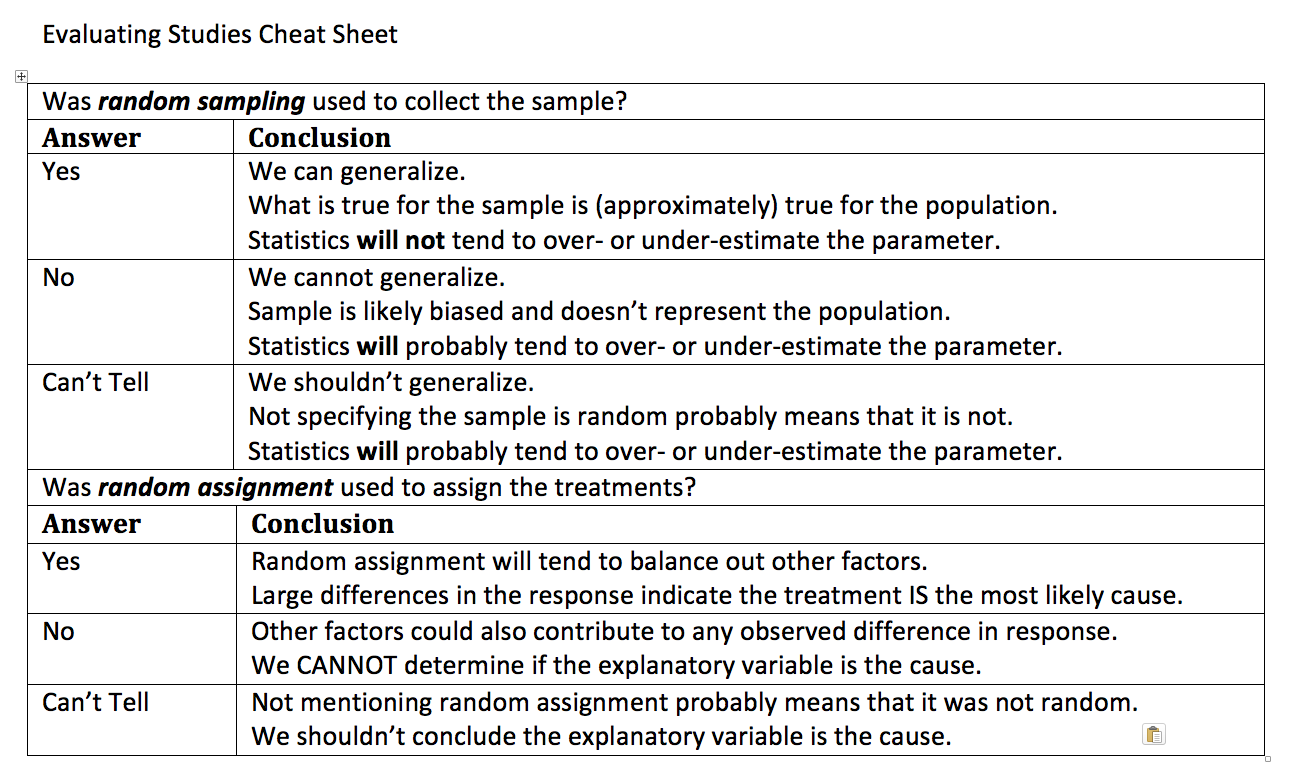
Evaluating studies cheat sheet

A study on flossing and gum disease (experiment)

A recent study was conducted to determine the effectiveness of flossing on gum disease. A group of 500 volunteers were randomly split into two groups. The first group was asked to floss once a day and the second group was asked to floss after each meal. Suppose that the group that flossed after every meal was much less likely to have gum disease as the group that flossed once per day.

(A) Yes
Note that the description mentioned that the participants were volunteers.
(B) No
The participants volunteered and were not randomly selected.

(A) Yes, the effects the flossing treatments would be the same for the general population.
The participants in the study were volunteers and not a randomly selected sample.
(B) No, there is a danger that our estimates of the effects of flossing on gum disease is likely biased.
The lack of a randomly selected sample means that we are in danger of biased estimates.

(A) Yes
(B) No
Note that the text mentions that the participants were randomly split into groups.

(A) Yes, the treatments are the only *likely* explanation for the differences.
Random assignment of the treatments will likely balance all other factors leading to gum disease.
(B) No, other factors are likely to have contributed to the difference.
Consider the effect of randomly assigning the flossing treatments on the other likely factors.

Another study on flossing and gum disease (observational study)

In another study on flossing and gum disease, a random sample of 500 people were surveyed on their flossing habits and whether or not they suffered from gum disease. Suppose that it was estimated that the people that flossed after every meal was much less likely to have gum disease as the group that flossed once per day.

(A) Yes
(B) No
The text explicitly mentioned a random sample.

(A) Yes, the effects the flossing treatments will be the same for the general population.
Because we are taking a random sample, our statistics should be unbiased and not over- or under-estimate the rates of gum disease in each group.
(B) No, there is a danger that our estimates of the effects of flossing on gum disease is likely biased.
What is the effect of random sampling on bias and a statistics ability to estimate a parameter?

(A) Yes
Note that the participants were not randomly assigned a flossing treatment, but were able to decide on their own flossing habits.
(B) No

(A) Yes, the differences in flossing habits of the participants are the only *likely* explanation for the differences.
The lack of random assignment of the treatments gives us no protection against other factors (like genetics) that effect gum disease.
(B) No, other factors are likely to have contributed to the difference.
The lack of random assignment of the treatments gives us no protection against other factors (like genetics) that effect gum disease.

1.5. Summarizing Data¶

Next, we will present some basic methods for summarizing data both numerically and graphically.

In particular, we will be looking to describe the distribution of the data, which consists of a list of feasible values for the data along with how often these values tend to occur. When describing a distribution, we will focus on answer four questions.

What is the shape of the distribution?
What is a typical value? (or equivalently) Where is the center of the distribution?
How are the values spread out?
Are there any outliers?

In the next few sections, we will cover graphical and numerical methods for answer these questions.

1.5.1. Graphing Distributions - Dot Plots and Histograms¶

Lecture on Graphs and the Shape of a Distribution

1.5.2. Shapes of a Distribution¶

One of the important features of a distribution is the shape of the distribution. In this class, we will describe the shape of the distribution in words using terms like symmetric, skewed left, skewed right, and bimodal.

Symmetric: A distribution is described as symmetric if portion of the graph to the left of the mean/average is approximately a mirror image of the portion of the graph to the right side of the mean/average.

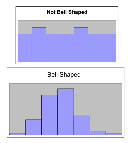
We will distinguish between symmetric graphs that are bell-shaped or not bell-shaped.

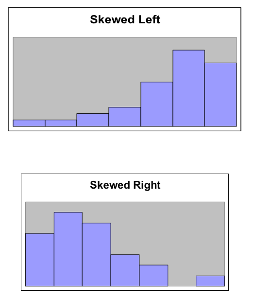
On the other hand, when a distribution is not symmetric, we focus on the tails of the distribution.

Skewed Left: A distribution is skewed left when it has a long left tail, that is its left tail is much longer than its right tail.
Skewed Right: A distribution is skewed right when it has a long right tail, that is its right tail is much longer than its left tail.

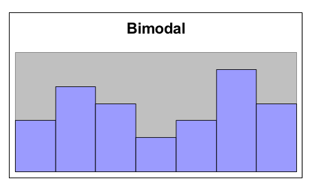
Finally, it is possible that we might have a graph with two peaks.

Bimodal: A distribution is bimodal if it has two distinct peaks. (The term bimodal literally means two modes, where a mode is a peak.)

(A) Symmetric
A symmetric graph has two tails that are about the same.
(B) Skewed left
A skewed left graph has a longer left tail.
(C) Skewed right
A skewed right graph has a longer right tail.

(A) Symmetric
A symmetric graph has two tails that are about the same.
(B) Skewed left
A skewed left graph has a longer left tail.
(C) Skewed right
A skewed right graph has a longer right tail.

(A) Symmetric
A symmetric graph has two tails that are about the same.
(B) Skewed left
A skewed left graph has a longer left tail.
(C) Skewed right
A skewed right graph has a longer right tail.

1.5.3. Measures of Center - Finding a Typical Value¶

Lecture on Measures of Center

Mean or Average: This is the (arithmetic) average of the data. It is calculated by adding all the values of the variable and dividing by the number of individuals.
Median: A value that splits the data into groups that consist of approximately half of the data. It is computed by (1) Putting the data in order and (2) Finding the middle value. If the data set has an even number of values, the average of the middle two values is used for the median.

While being able to compute the value of a summary statistic is important, *it is even more important to understand what each number tells us about the distribution. Here are the standard interpretations for these statistics.

Standard Interpretation of the Mean

The mean is the balance point or center of mass of the distribution, that is, it is the location at which the dot plot would balance on your finger.

Standard Interpretation of the Median

The median splits the data in half. Approximately 50% of the data will be above and below the median. (The only situation where this is not exactly 50% is when there are multiple values stacked at the median.)

Q-39: The following values are the serum cholesterol levels (mg/dLi) of six men with high cholesterol.

366 327 230 274 292 274

Compute the mean of these data.

(A) 252.0
You need to add up all the values and divide by the number of individuals.
(B) 283.0
You need to add up all the values and divide by the number of individuals.
(C) 293.8

Q-40: The following values are the serum cholesterol levels (mg/dLi) of six men with high cholesterol.

366 327 230 274 292 274

Compute the median of these data.

(A) 252.0
Make sure you reorder the data, *then* find the middle value.
(B) 283.0
(C) 293.8
Sort the data and find the middle value.

1.5.4. Measures of Spread - Finding the Amount of Concentration or Spread¶

Lecture on Measures of Spread

In an earlier section, we took on the task of determining a “typical value”. The answer was to use a measurement in the center of the distribution of like the mean and median. Unfortunately, knowing the location of the center of the distribution is not enough information.

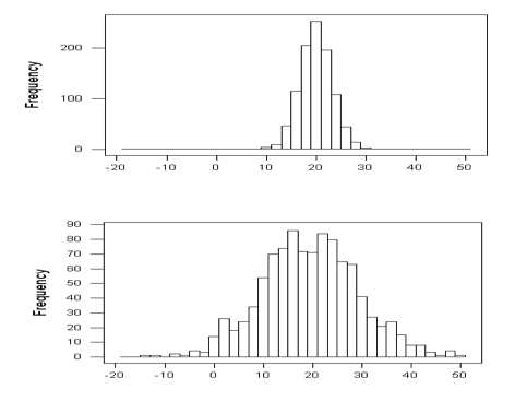
For example, the two graphs shown above have centers that are very similar, but one graph has data that is more concentrated than another. This difference is very important in many fields. In manufacturing, creating products that are very similar can reduce waste, and in statistics, having estimates that are more concentrated, or less spread out, means that we are making better guesses.

The most basic measurement of spread is the range of the data.

Range: The difference/distance between the largest and smallest value in the data set.

Unfortunately, the range is very susceptible to outliers, making it a poor measure of spread. We will instead use two other measures of spread, the interquartile range (IQR) and the standard deviation (from the mean).

(A) The difference between the smallest and largest values in the data.
This is the range of the data.
(B) The distance between a typical/average value and the mean.
(C) The the range of the middle 50% of the data.
This is the interquartile range.

Interquartile range (IQR): The range of the middle 50% of the data. It is found by (a) finding the medians of the lower and upper halves of the data, called Q1 and Q3, respectively. Then the IQR = Q3 - Q1.
Standard Deviation (SD): The standard deviation is computed using the formula given below. It can be thought of as the distance of a typical/average value to the mean.

\[SD = \sqrt{\frac{\sum (x - \bar{x})^2}{n-1}}\]

For both statistics, the value indicates how concentrated or spread out the data is.

A larger value of the SD or IQR means that the data is more spread out.
A smaller value of the SD or IQR means that the data is more concentrated.

As mentioned earlier, understanding how to interpret the value of a statistic is perhaps more important than being able to compute the value. Here are the standard interpretations of each of these statistics.

Standard Interpretation of the Standard Deviation

The standard deviation tells us how far a typical value is from the mean.

Standard Interpretation of the Interquartile Range

The interquartile range measures the spread of the middle 50% of the data.

Resistance

The IQR is more resistant to the effects of outliers than the standard deviation.

(A) The difference between the smallest and largest values in the data.
(B) The distance between a typical/average value and the mean.
(C) The range of the middle 50% of the data.

(A) The difference between the smallest and largest values in the data.
(B) The distance between a typical/average value and the mean.
(C) The range of the middle 50% of the data.

1.6. Unusual Values and the p-Value¶

Lecture on p-values

We will spend a considerable amount of time in this course trying to decide if a value is unusually large or unusually small. For example, if we were trying to determine if the hiring practices in a school district are discriminatory, we will need to determine if the school hires an unusually low number of African-American teachers.

Before we can determine if a value is unusual, we need a good definition of what it means to be unusually large or unusually small in a statistical sense.

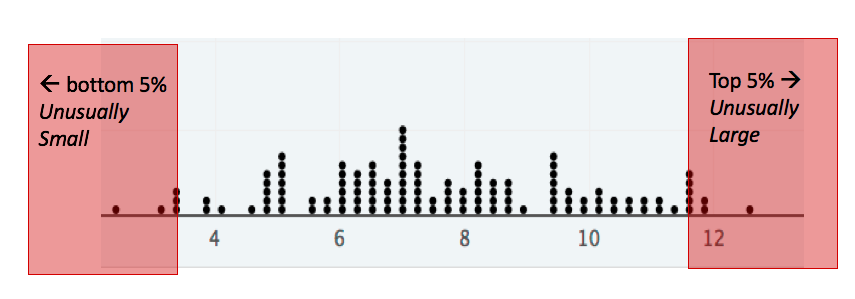
Unusually large values: A value is considered unusually large if it is in the largest 5% of the distribution.
Unusually small values: A value is considered unusually small if it is in the smallest 5% of the distribution.

Note

There is nothing special about picking 5%, and in fact later in the course we will see that adjusting this value gives us some control over a certain type of error. For now, we will stick to 5% and call this the 5% rule.

Now that we know what it means to be unusually large or small, we need a method of determining if a specific value of interest is unusually large. For example, I have a friend that is 78 inches tall (6’ 6”). I know that he is fairly tall, but is he unusually tall, in the statistical sense?

When answering this question intuitively, I believe that it is natural to compare my friend to other tall people, asking What percentage of the time do I meet men that is 78 inches tall or taller. This is the exact intuition that leads to our definition of an upper p-value.

On the other hand, we might ask if someone that is 63.5 inches tall, like my wife, is unusually short. Again in a statistical sense. This time it is natural to compare someone on the small side of the distribution with other small values, leading to what I like to call a lower p-value.

Upper p-value: The upper p-value of a given value x is the proportion of the distribution that is at or above the value. This measurement is useful in determining if a value is unusually large.
Lower p-value: The lower p-value of a given value x is the proportion of the distribution that is at or below the value. This measurement is useful in determining if a value is unusually small.

1.6.1. Example: Using a lower p-value to determine if 4 is unusually small.¶

Consider the distribution shown below. There are 117 dots on the graph, and we want to answer the question Is the value 4 unusually small. Because we are focusing on small values, we will use a lower p-value, because it makes sense to compare a potentially small value to other small values. There are 7 dots that are at or below 4, so the lower p-value of 4 rounds up to 0.06 or 6%. Since there is more than 5% of the distribution below 4, 4 is not in the smallest 5% of the distribution and therefore is not unusually small.

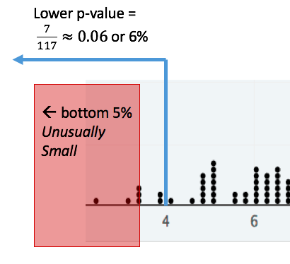
Thus, a value is only unusually small if its lower p-value is smaller than 5% (when using the 5% rule). The same is true for an upper p-value.

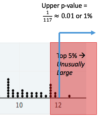
1.6.2. Example: Using an upper p-value to determine if 12 is unusually large.¶

This time, consider the question Is 12 unusually large? In this case the upper p-value is a little less than 1%. Since less than 5% of the distribution is above 12, we see that

12 is in the largest 1%, and

12 is unusually large, according to the 5% rule.

(A) lower p-value.
When looking at a potentially small value, compare it to other small values.
(B) upper p-value.
Focus on the smallest part of the distribution, i.e. the left tail.

(A) lower p-value.
Focus on the largest part of the distribution, i.e. the right tail.
(B) upper p-value.
When looking at a potentially large value, compare it to other large values.

(A) Yes
If the lower p-value is smaller than 5%, the value is in the smallest 5% and thus unusually smallest.
(B) No
Consider the fact that the value has only 2.3% of the distribution below it. Is it in the smallest 5% of the distribution?

(A) Yes
Consider the fact that the value more than 12.7% of the distribution above it. Is it in the largest 5% of the distribution?
(B) No
If the upper p-value is larger than 5%, the value is NOT in the largest 5% and thus NOT unusually large.

General P-value Rule

A value is unusually small when the lower p-value is less than 5% (when using the 5% rule).

A value is unusually large when the upper p-value is less than 5% (when using the 5% rule).

In both cases, small p-values mean unusual values.

1. Introduction to Data¶

1.1. All about data¶

1.1.1. Understanding Data Individually¶

1.1.2. Understanding Data Collectively¶

1.1.3. Summarizing Data Numerically¶

1.1.4. Types of Variables¶

1.2. Sources of Bias¶

1.3. Types of Studies¶

1.4. Evaluating Studies¶

1.5. Summarizing Data¶

1.5.1. Graphing Distributions - Dot Plots and Histograms¶

1.5.2. Shapes of a Distribution¶

1.5.3. Measures of Center - Finding a Typical Value¶

1.5.4. Measures of Spread - Finding the Amount of Concentration or Spread¶

1.6. Unusual Values and the p-Value¶

1.6.1. Example: Using a lower p-value to determine if 4 is unusually small.¶

1.6.2. Example: Using an upper p-value to determine if 12 is unusually large.¶