3.8. Computational Complexity and Big O Notation.¶

3.8.1. Formal definition¶

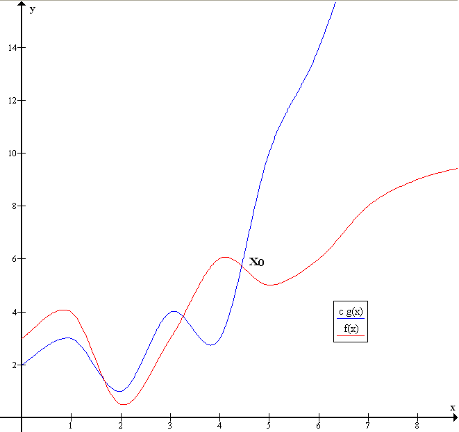
Let \(f\) and \(g\) be two functions defined on some subset of the real numbers. One writes

if and only if there is a positive constant \(M\) such that for all sufficiently large values of \(x\), the absolute value of \(f(x)\) is at most \(M\) multiplied by the absolute value of \(g(x)\). That is, \(f(x)=O(g(x))\) if and only if there exists a positive real number \(M\) and a real number \(x_0\) such that

In many contexts, the assumption that we are interested in the growth rate as the variable \(x\) goes to infinity is left unstated, and one writes more simply that

This image illustrates the formal definition of the Big O notation. The function \(cg\) is an upper bound for \(f\) for all values larger than \(x_0\), so we say \(f(x)=O(g(x))\). Image Source

3.8.2. Example¶

In typical usage, the formal definition of \(O\) notation is not used directly; rather, the \(O\) notation for a function \(f\) is derived by the following simplification rules:

• If \(f(x)\) is a sum of several terms, if there is one with largest growth rate, it can be kept, and all others omitted.
• If \(f(x)\) is a product of several factors, any constants (terms in the product that do not depend on \(x\)) can be omitted.

For example, let \(f(x) = 6x^4 − 2x^3 + 5\), and suppose we wish to simplify this function, using \(O\) notation, to describe its growth rate as \(x\) approaches infinity. This function is the sum of three terms: \(6x^4\), \(2x^3\), and 5. Of these three terms, the one with the highest growth rate is the one with the largest exponent as a function of \(x\), namely \(6x^4\). Now one may apply the second rule: \(6x^4\) is a product of 6 and \(x^4\) in which the first factor does not depend on \(x\). Omitting this factor results in the simplified form \(x^4\). Thus, we say that \(f(x)\) is a “big-oh” of \((x^4)\). Mathematically, we can write \(f(x)=O(x^4)\). One may confirm this calculation using the formal definition: let \(f(x)=6x^4 − 2x^3 + 5\) and \(g(x)=x^4\). Applying the formal definition from above, the statement that \(f(x)=O(x^4)\) is equivalent to its expansion, \(|f(x)| \le \; M |x^4|\) for some suitable choice of \(x_0\) and \(M\) and for all \(x > x_0\). To prove this, let \(x_0=1\) and \(M=13\). Then, for all \(x > x_0\)

so

3.8.3. Infinite asymptotics¶

Big O notation is useful when analyzing algorithms for efficiency. For example, the time (or the number of steps) it takes to complete a problem of size \(n\) might be found to be \(T(n) = 4n^2 − 2n + 2\). As \(n\) grows large, the \(n^2\) term will come to dominate, so that all other terms can be neglected—for instance when \(n = 500\), the term \(4n^2\) is 1000 times as large as the \(2n\) term. Ignoring the latter would have negligible effect on the expression’s value for most purposes. Further, the coefficients become irrelevant if we compare to any other order of expression, such as an expression containing a term \(n^3\) or \(n^4\). Even if \(T(n) = 1,000,000n^2\), if \(U(n) = n^3\), the latter will always exceed the former once \(n\) grows larger than 1,000,000 (\(T(1,000,000) = 1,000,000^3= U(1,000,000)\)). Additionally, the number of steps depends on the details of the machine model on which the algorithm runs, but different types of machines typically vary by only a constant factor in the number of steps needed to execute an algorithm. So the big O notation captures what remains: we write either

or

and say that the algorithm has \(order of n^2\) time complexity. Note that “=” is not meant to express “is equal to” in its normal mathematical sense, but rather a more colloquial “is”, so the second expression is sometimes considered more accurate (see the ” Equals sign ” discussion below) while the first is considered by some as an Abuse of notation.

This image compares the rate of growth for functions from various Big O classes. Eventually functions from the same class tend to grow at similar rates and all members of one class tend to dominate functions from a lower-order group. Image Source

3.8.4. Properties¶

If the function \(f\) can be written as a finite sum of other functions, then the fastest growing one determines the order of \(f(n)\). For example

In particular, if a function may be bounded by a polynomial in \(n\), then as \(n\) tends to \(\infty\), one may disregard lower-order terms of the polynomial. Another thing to notice is the sets \(O(n^c)\) and \(O(c^n)\) are very different. If \(c\) is greater than one, then the latter grows much faster. A function that grows faster than \(n^c\) for any \(c\) is called superpolynomial. One that grows more slowly than any exponential function of the form \(c^n\) is called subexponential. An algorithm can require time that is both superpolynomial and subexponential; examples of this include the fastest known algorithms for integer factorization and the function \(n^log n\).

We may ignore any powers of \(n\) inside of the logarithms. The set \(O(\log n)\) is exactly the same as \(O(\log(n^c))\). The logarithms differ only by a constant factor (since \(\log(n^c) = c (\log n)\)) and thus the big O notation ignores that. Similarly, logs with different constant bases are equivalent. On the other hand, exponentials with different bases are not of the same order. For example, \(2^n\) and \(3^n\) are not of the same order.

Changing units may or may not affect the order of the resulting algorithm. Changing units is equivalent to multiplying the appropriate variable by a constant wherever it appears. For example, if an algorithm runs in the order of \(n^2\), replacing \(n\) by \(cn\) means the algorithm runs in the order of \(c^2n^2\), and the big O notation ignores the constant \(c^2\). This can be written as \(c^2n^2 = O(n^2)\). If, however, an algorithm runs in the order of \(2^n\), replacing \(n\) with \(cn\) gives \(2^{cn} = (2^c)^n\). This is not equivalent to \(2^n\) in general. Changing variables may also affect the order of the resulting algorithm. For example, if an algorithm’s run time is \(O(n)\) when measured in terms of the number \(n\) of digits of an input number \(x\), then its run time is \(O(\log x)\) when measured as a function of the input number \(x\) itself, because \(n=O(\log x)\).

Product

Sum

This implies

and if \(f\) and \(g\) are positive functions, \(f + O(g) = O(f + g).\)

Multiplication by a constant

Let \(k\) be a constant. Then \(O(k g) = O(g)\) if \(k\) is nonzero.

In the next section, we will consider the computational complexity of various operations on Python lists.

3.8.5. The computational complexity of the find method¶

In this section, we will look at the run-time complexity of the find method of a list or a string. For a list, we are interested in the order of growth of the find method as the length of the sequence \(n\) grows without bound and we will classify this rate using Big O notation. When looking at orders of growth for an algorithm as the it is common to consider the worst-case and the average case.

Worst Case

In the worst case, the item that we are searching for is at the end of the sequence, and it will take \(n\) steps to find the value. Thus the worst-case order of the find method is \(O(n)\).

Average Case

When thinking of the “average-case”, we imagine applying the find method to randomly shuffled lists. In the average case, the item that we are searching for be in the middle of the sequence, and it will take (about) \(\frac{n+1}{2}\) steps to find the value. Thus the average-case order of the find method is \(O\left(\frac{n}{2}+\frac{1}{2}\right)= O(n)\).

3.8.6. The computational complexity of item lookup¶

Now consider the order of growth of the indexing operator. Recall that Python lists are really a list of references to other objects in memory. This means that a list really holds a list of memory addresses, e.g. which will be either 32 or 64 bits of data (depending on machine architecture and machine language.)

L = [ADDRESS_0, ADDRESS_1, ..., ADDRESS_(n-1)]

These addresses will all be the same size, getting the address for the value are index k consists of adding some multiple of k to the first address.

L[k] returns ADDRESS_k = ADDRESS_0 + M*k

This means that, regardless of the length of the list L, we can return the value at any index with one arithmetic computation. In other words, indexing on lists and strings is \(O(1)\).

L[0] returns ADDRESS_0 = ADDRESS_1 + M*0

3.8.7. The complexity of the slice operator¶

The complexity of the slice operator is a little more complicated and depends on the rate at which the range of values in the slice grow. Recall that the slice returns a new list, which means that we will need to construct a new list of references to these values.

L[i:k] returns [ADDRESS_i, ADDRESS_(i+1), ..., ADDRESS_k]

We will consider a number of examples, but the questions of the complexity of the slice operator needs to be considers on a case-by-case basis.

Slice of a constant length

Suppose that our slice is of the form L[i:i+c] for some constant c. To construct a slice of constant length, we need to

1. allocate memory for the new list (\(O(1)\))
2. copy or compute the c memory addresses. (\(O(c) = O(1)\))

Thus, the complexity of the slice of constant length is \(O(1) + O(1) = O(1)\).

Slice all but the first item c items

Suppose that our slice is of the form L[c:] for some constant c and assume that len(L) = n. In this case, the size of the slice grows at the same rate as the original list. To construct this type of slice, we need to

1. allocate memory for the new list (\(O(1)\))
2. copy or compute the n - c memory addresses. (\(O(n - c) = O(n)\))

Thus, the complexity of the slice of this type is \(O(n) + O(1) = O(n)\). Finally, we note that this case includes L[:], i.e. using the slice operator to copy the entire list.

3.8.8. Append versus Concatenate¶

The append method adds a new item to the end of a list. It is also possible to add a new item to the end of a list by using the concatenation operator. However, you need to be careful.

Consider the following example. The original list has 3 integers. We want to add the word “cat” to the end of the list.

Here we have used append which simply modifies the list. In order to use concatenation, we need to write an assignment statement that uses the accumulator pattern:

origlist = origlist + ["cat"]

Note that the word “cat” needs to be placed in a list since the concatenation operator needs two lists to do its work.

It is also important to realize that with append, the original list is simply modified. On the other hand, with concatenation, an entirely new list is created. This can be seen in the following codelens example where newlist refers to a list which is a copy of the original list, origlist, with the new item “cat” added to the end. origlist still contains the three values it did before the concatenation.

This distinction has an impact on the complexity of these two operations. For a list of length n, the concatenation operation will be \(O(n)\) (This is equivalent to origlist[:] + ["cat"] which is \(O(n) + O(1) = O(n)\).)

When Python constructs a new list, it actually allocates extra memory in anticipation of future calls to append. So the complexity of an append statement, depends on whether or not this extra memory is still available. In the case that we have exosted the memory, we will need to allocate more memory and copy the list (\(O(n)\)), but it the memory is available, we just need to copy the memory address of the new element into the next memory slot (\(O(1)\)). Luckily, Python allocates memory is such a way that the need to add memory and copy the list happens to infrequently, we can consider append to have an amortized worst case of \(O(1)\)

Check you understanding

rec-5-21: What is printed by the following statements?

alist = [4, 2, 8, 6, 5]
alist = alist + 999
print(alist)

• (A) [4, 2, 8, 6, 5, 999]
• You cannot concatenate a list with an integer.
• (B) Error, you cannot concatenate a list with an integer.
• Yes, in order to perform concatenation you would need to write alist+[999]. You must have two lists.

3.8.9. Summary of Computational Complexity for Lists and Strings¶

In this section, we looked at the complexity of various operations on lists and strings. When selecting a data structure for your program, it is important to consider the operations that you will perform and select the best data structure for that job. We have seen that Python lists and strings excel at indexing, but are not necessarily great at looking up values. In a future chapter, we will introduce two Python data structures that are much more efficient when it comes to look-up operations.