1.1. Why Python?
Source
This section is a modified version of the SciPy notes that can be found here. Authors: Fernando Perez, Emmanuelle Gouillart, Gaël Varoquaux, Valentin Haenel
1.1.1. The scientist’s needs
When working with data, a data scientist needs to be able to
- Get data (simulation, experiment control),
- Manipulate and process data,
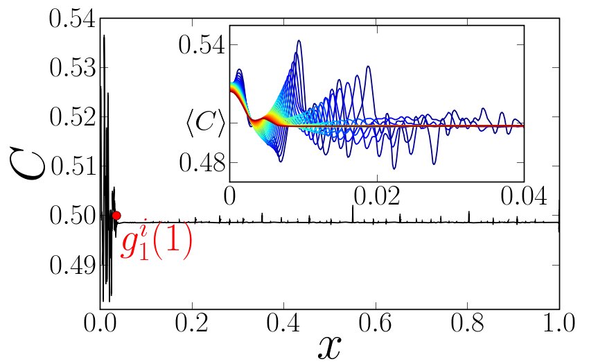
- Visualize results, quickly to understand, but also with high quality figures, for reports or publications.
The Python programming language is a popular tool for data scientists, due to its interactive, dynamic nature and a powerful and plentiful library of tools for many tasks.
1.1.2. Python’s strengths
- Batteries included Rich collection of already existing bricks of classic numerical methods, plotting or data processing tools. We don’t want to re-program the plotting of a curve, a Fourier transform or a fitting algorithm. Don’t reinvent the wheel!
- Easy to learn Most scientists are not paid as programmers, neither have they been trained so. They need to be able to draw a curve, smooth a signal, do a Fourier transform in a few minutes.
- Easy communication To keep code alive within a lab or a company it should be as readable as a book by collaborators, students, or maybe customers. Python syntax is simple, avoiding strange symbols or lengthy routine specifications that would divert the reader from mathematical or scientific understanding of the code.
- Efficient code Python numerical modules are computationally efficient. But needless to say that a very fast code becomes useless if too much time is spent writing it. Python aims for quick development times and quick execution times.
- Universal Python is a language used for many different problems. Learning Python avoids learning a new software for each new problem.
1.1.3. How does Python compare to other solutions?
Python is not the only choice for working with data and below we compare and contrast the pros and cons of many popular options.
1.1.3.1. Compiled languages: C, C++, Fortran...
| Pros: |
|
|---|---|
| Cons: |
|
1.1.3.2. Matlab scripting language
| Pros: |
|
|---|---|
| Cons: |
|
1.1.3.3. Julia
| Pros: |
|
|---|---|
| Cons: |
|
1.1.3.4. Other scripting languages: Scilab, Octave, R, IDL, etc.
| Pros: |
|
|---|---|
| Cons: |
|
1.1.3.5. Python
| Pros: |
|
|---|---|
| Cons: |
|
1.1.3.5.1. The Scientific Python ecosystem
Unlike Matlab, or R, Python does not come with a pre-bundled set of modules for scientific computing. Below are the basic building blocks that can be combined to obtain a scientific computing environment:
Python, a generic and modern computing language
- The language: flow control, data types (
string,int), data collections (lists, dictionaries), etc. - Modules of the standard library: string processing, file management, simple network protocols.
- A large number of specialized modules or applications written in Python: web framework, etc. ... and scientific computing.
- Development tools (automatic testing, documentation generation)
Core numeric libraries
- Numpy: numerical computing with powerful numerical arrays objects, and routines to manipulate them. http://www.numpy.org/
- Scipy : high-level numerical routines. Optimization, regression, interpolation, etc http://www.scipy.org/
- Matplotlib : 2-D visualization, “publication-ready” plots http://matplotlib.org/
Advanced interactive environments:
- IPython, an advanced Python console http://ipython.org/
- Jupyter, notebooks in the browser http://jupyter.org/
Domain-specific packages,
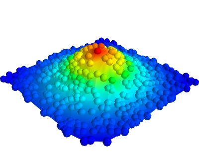
- Mayavi for 3-D visualization
- pandas, statsmodels, seaborn for statistics
- sympy for symbolic computing
- scikit-image for image processing
- scikit-learn for machine learning
and many more packages not documented in the scipy lectures.
In [1]: import numpy as np

In [1]: np.random.seed(4)
1.1.3.5.2. Before starting: Installing a working environment
Python comes in many flavors, and there are many ways to install it. However, we recommend to install a scientific-computing distribution, that comes readily with optimized versions of scientific modules.
Under Linux
If you have a recent distribution, most of the tools are probably packaged, and it is recommended to use your package manager.
Other systems
There are several fully-featured Scientific Python distributions:
Python 3 or Python 2?
In 2008, Python 3 was released. It is a major evolution of the language that made a few changes. Some old scientific code does not yet run under Python 3. However, this is infrequent and Python 3 comes with many benefits. We advise that you install Python 3.
In this course, we will be using the Anaconda distribution of Python 3, as it has most of the important modules needed by a data scientist. Be sure to download and install this package before proceeding with the rest of the book.
1.1.3.5.3. The workflow: interactive environments and text editors
Interactive work to test and understand algorithms: In this section, we describe a workflow combining interactive work and consolidation.
Python is a general-purpose language. As such, there is not one blessed environment to work in, and not only one way of using it. Although this makes it harder for beginners to find their way, it makes it possible for Python to be used for programs, in web servers, or embedded devices.
1.1.4. Interactive work
We recommend an interactive work with the IPython console, or its offspring, the Jupyter notebook. They are handy to explore and understand algorithms. In this section, we will highlight some useful features of the IPython console.
IPython includes some useful shortcuts for getting documentation and help. We can use the ? and ?? operators after an object:
In [1]: print?
  File "<ipython-input-1-3b91d809f69e>", line 2
    bookmark -d ipy_savedir
                          ^
SyntaxError: invalid syntax
In [2]: print??
Type: builtin_function_or_method
1.1.5. Elaboration of the work in an editor
As you move forward, it will be important to not only work interactively, but also to create and reuse Python files. For this, a powerful code editor will get you far. Here are several good easy-to-use editors:
Some of these are shipped by the various scientific Python distributions, and you can find them in the menus. For this course, we will focus on using the PyCharm IDE, which is freely available for academic use.
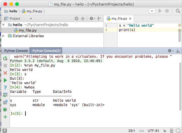
As an exercise, create a file my_file.py in a code editor, and add the following lines:
s = 'Hello world'
print(s)
Now, you can run it in IPython console or a notebook and explore the resulting variables:
In [1]: %run my_file.py
Hello world

In [2]: s
Out[2]: 'Hello world'

In [3]: %whos
Variable   Type    Data/Info
----------------------------
s          str     Hello world
Here is what this looks like in PyCharm.
From a script to functions
While it is tempting to work only with scripts, that is a file full of instructions following each other, do plan to progressively evolve the script to a set of functions:
- A script is not reusable, functions are.
- Thinking in terms of functions helps breaking the problem in small blocks.
1.1.6. IPython and Jupyter Tips and Tricks
The user manuals contain a wealth of information. Here we give a quick introduction to four useful features: history, tab completion, magic functions, and aliases.
Command history Like a UNIX shell, the IPython console supports command history. Type up and down to navigate previously typed commands:
In [1]: x = 10

In [2]: <UP>

In [2]: x = 10
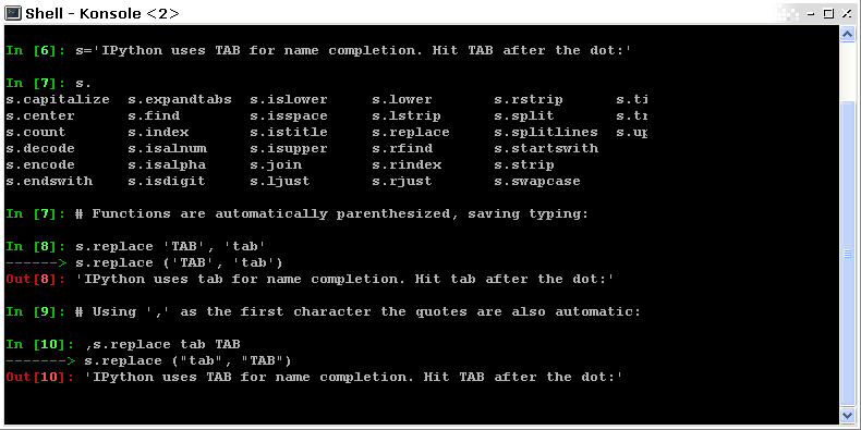
Tab completion Tab completion, is a convenient way to explore the structure of any object you’re dealing with. Simply type object_name.<TAB> to view the object’s attributes. Besides Python objects and keywords, tab completion also works on file and directory names.*
In [1]: x = 10

In [2]: x.<TAB>
x.bit_length   x.denominator  x.imag         x.real
x.conjugate    x.from_bytes   x.numerator    x.to_bytes
Magic functions
The console and the notebooks support so-called magic functions by prefixing a command with the
% character. For example, the run and whos functions from the
previous section are magic functions. Note that, the setting automagic,
which is enabled by default, allows you to omit the preceding % sign. Thus,
you can just type the magic function and it will work.
Other useful magic functions are:
%cdto change the current directory.In [1]: cd /tmp /tmp
%cpasteallows you to paste code, especially code from websites which has been prefixed with the standard Python prompt (e.g.>>>) or with an ipython prompt, (e.g.in [3]):In [2]: %cpaste Pasting code; enter '--' alone on the line to stop or use Ctrl-D. :>>> for i in range(3): :... print(i) :-- 0 1 2
%timeitallows you to time the execution of short snippets using thetimeitmodule from the standard library:In [3]: %timeit x = 10 10000000 loops, best of 3: 39 ns per loop
%debugallows you to enter post-mortem debugging. That is to say, if the code you try to execute, raises an exception, using%debugwill enter the debugger at the point where the exception was thrown.In [4]: x === 10 File "<ipython-input-6-12fd421b5f28>", line 1 x === 10 ^ SyntaxError: invalid syntax In [5]: %debug > /.../IPython/core/compilerop.py (87)ast_parse() 86 and are passed to the built-in compile function.""" ---> 87 return compile(source, filename, symbol, self.flags | PyCF_ONLY_AST, 1) 88 ipdb>locals() {'source': u'x === 10\n', 'symbol': 'exec', 'self': <IPython.core.compilerop.CachingCompiler instance at 0x2ad8ef0>, 'filename': '<ipython-input-6-12fd421b5f28>'}
Aliases
Furthermore IPython ships with various aliases which emulate common UNIX
command line tools such as ls to list files, cp to copy files and rm to
remove files (a full list of aliases is shown when typing alias).
Getting help
- The built-in cheat-sheet is accessible via the
%quickrefmagic function. - A list of all available magic functions is shown when typing
%magic.
%quickref
%magic