2.3. Expressions, Values and Evaluation
The focus of this chapter has been using expressions in python to perform
computations. We have seen that we can use lambda expressions to save
expressions for later computation and the conditional expression to decide
branch between two expressions depending on some condition.
Here is an outline of a formal definition the expressions seen so far.
Definition of Expressions (so far)
An expression (EXPR for short) consists of
- values: 5, “1”, True, ...
- operations: EXPR1 OP EXPR2, where OP is any operator (+, -, and, ==, etc.)
- conditional expressions: EXPR1 if EXPR2 else EXPR3
- lambda expressions: lambda VAR: EXPR (special type of value)
- function application: EXPR(EXPR)
This is an example of a recursive definition as we are using the term being defined (expression or EXPR) as part of the definition. Recursive definitions lead to structures that can be thought of as a tree, and in the case of our expressions, the end of every branch in the tree will be a value.
At this point, you may be wondering why there is so much focus on expressions. Expressions are the building blocks for functional programs and using the right expressions can lead to programs that are easier to understand. In particular, part of a program is referentially transparent if it can be replaced with it’s value without changing the meaning of the program, making it easier to understand. Expressions constructed out of lambda expressions, conditional expressions and operations will be referentially transparent.
For example, the expression 1+1 is referentially transparent, because it can
be replaced with its value 2 without changing the program in any way. On
the other hand, a call to the print function is not referentially
transparent. print is an example of a void function, a function that
returns no (meaningful) value. In Python, all functions actually return
something and void functions return None, a special value that stands in for
nothing. We can verify that print returns None using the is
comparison.
In [1]: print("Hi") is None
The problem with print, in terms of referential transparency, is that it is
side-effecting. For our purposes, a side-effect is any effect of a
function that can’t be determined looking at the input and output. In the case
of print, the side effect is printing some text to the screen. Replacing a
print function with its value of None clearly changes the Hello
World program, illustrating the fact that print is not referentially
transparent.
In [1]: print("Hello World")

# Replace print with its value None
In [1]: None

# Not the same program!
2.3.1. What is Evaluation?
When we type an expression into the Python (or IPython) interpreter, it is converted to a value. The process of converting expressions to values is called evaluation.
Evaluation of values and operations is fairly obvious. The result of evaluating
a value is that value. The evaluation of an operation such as EXPR = EXPR1 OP
EXPR2 is also easy to understand. We simply follow our order of operation by
evaluating EXPR1 and EXPR2, then apply the operation to the resulting
values.
To understand the evaluation of lambda expressions, we will need to understand two related topics: closures and the scope of a variable.
2.3.2. Lambda Expressions and Closures
The lambda expressions that we created so far have been pretty simple. Note
that the body of a lambda expression is also an expression. Consequently lambda
expressions can be embedded in the body of another lambda expression. For
example, another way to generalize the apply_tax function is to create
another function make_apply_tax that takes the tax rate as input and returns
a lambda expression that uses this rate.
In [1]: make_apply_tax = lambda rate: lambda cost: rate*cost
We have created a function that returns another function. Such a function is
called a higher-order function and we will look at these types of function in
more depth in a later chapter. The make_apply_tax function is a
function factory, used to create specialize functions. When working on a
specific example, we will call make_apply_tax to create a specialized
version of apply_tax for that problem.
In [1]: rate = 1.065

In [1]: apply_tax = make_apply_tax(rate)

In [1]: type(apply_tax)

In [1]: apply_tax(1)

In [1]: apply_tax(4.55)
Let’s examine this program in codelens.
(closures1)
Step through the program until line 3 is evaluated (steps 4 through 7). Notice
that the apply_tax function is saved as f1. Moreover, the function
apply_tax is bundled with the specific value of rate (1.065) used at the
time of creation. This is an example of a closure, where a function bundled
the outside values that it references.
Designing functions as closures allows us to create multiple versions of
apply_tax simultaneously.
(closures2)
In this example, we see that each of the apply_tax functions is bundled with
the appropriate value and the second call to make_apply_tax did not affect
the first call in any way. This explains, in detail, how Python evaluates
nested lambda expressions: a value is placed in memory that includes the
function plus the value of any outer variable referenced in the body. This type
of value is known as a closure. Next, we consider the evaluation of a function
call. It turns out that the choice of order of this evaluation illustrate the
distinction between lazy evaluation and strict evaluation.
There are two more subtle implementation details that we need to understand before we can understand the evaluation of functions and function calls in Python. In the next section, we look at when Python creates a closure and how Python resolves local and global variables.
2.3.3. Closure creation and the resolution of global and local variables
Python functions are not always closures and whether or not Python creates a closure depends on whether or not the function references a local variable bound outside its scope. Consider the following example.
(closures3)
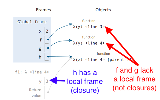
In the above example, the first two function are not closures but the third function is. Function that are not closures do not get their own frame of reference, where as a closure does. This is illustrated in the following figure.

In this figure, we see that the first two functions lack their own frame-of-reference and are not closures. On the other hand, the third function contains a local frame that contains the value ofyand is a closure.
Python’s evaluation rules are different for references to global variables (variables defined in the main namespace) and local variables defined outside a function’s body. If a function does not reference any local variable outside of its scope, it won’t be a closure. Furthermore, references to global variables have dynamic resolution, meaning the value of the variable is resolved at run-time, not at the creation of the function.
In the above example shown in codelens, we see that the third function h has
a reference to a bound local variable outside its scope, namely y.
Furthermore, the value that is referenced in this local frame is the value of
y when h was created. This method of resolving a variable is known as
lexical resolution. References to global variables have a different method
of resolution in Python.
(closures4)
In this last example, we see that the value of x used in the calculation of
result was 4 and not 2. This indicates that references to global variables
are resolved at run-time using the current state of the function at the time of
the function call. This type of resolution is known as dynamic resolution.
2.3.4. Variable Scope and Substitution
The ability to nest lambda expressions brings about another problem. Consider the following expression.
lambda x: lambda x: x**2
The body of the outer function is a lambda function and the body of the inner
function is x**2, but which x is this body referring to, the outer
parameter or the inner parameter? Let’s runs some code to find out, where we
have added another wrinkle by introducing a global variable x as well.
In [1]: x = 1

In [1]: f = lambda x: lambda x: x**2

# Calling the outer function returns a function
In [1]: g = f(2)

In [1]: type(g)

In [1]: g(3)
If x**2 referred to the outer parameter, we would have seen 2**2 = 4 as
the value of g(3). Similarly, if x was referring to the global
variable, g(3) would return 1**2 = 1. So clearly the
x in the expression x**2 is referring to the inner x parameter.
What is going on here? The answer has to do with a variables scope. Recall
that variables, whether constructed through an assignment statement or function
call, are bound to values. The (lexical) scope of a variable is the portion
of the code for which that variable represents it’s value. In other words, if a
variable x is bound to 5, the scope is all parts of the code where
evaluating x will return 5.
Run the same program in codelens and see if things clear up.
(scope1)
Functions and lambda expression complicate the issue, as their parameters are local variables, meaning that their scope is restricted to the body of the function or expression.
So what happens if we use the same name for a parameter in nested lambda
expressions? The value bound to x changes based on the scope of the
variable, using the value from the most local x variable. The following
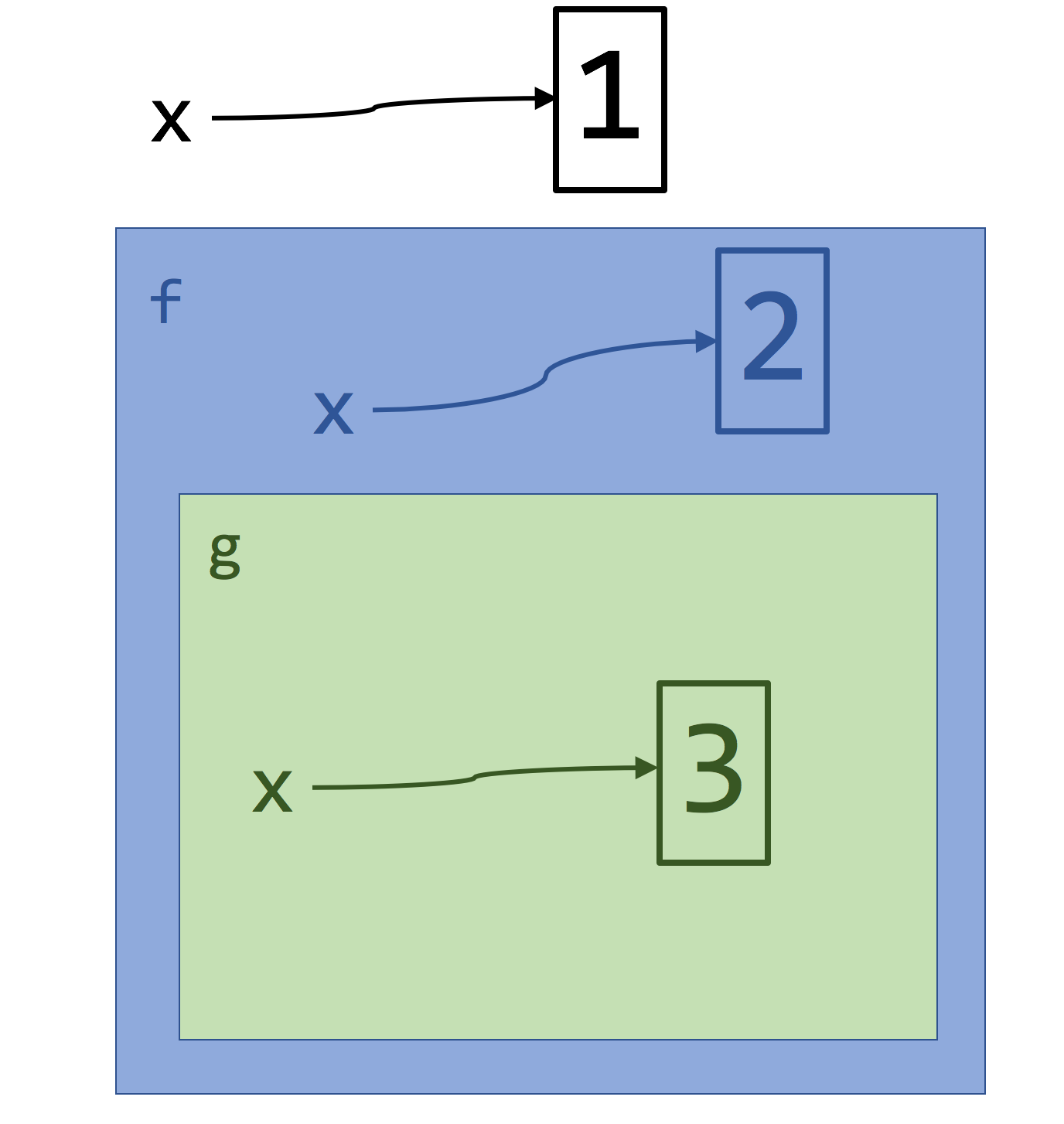
figure illustrates the scope of all three x variables.

x, which is bound to the the argument of g(3),
namely 3. The scope of the inner most x is the body of the inner
lambda. The outer parameter gets bound to 2, and the scope of this variable
is inside the body of the outer function, but not in the body of the inner
lambda. The global variable has a scope that consists of the global name
space but is over-ridden in the body of both functions.Ideally, we would like to think about evaluation of referentially transparent expressions using substitution: replace each expression with the right value. But substitution becomes tricky when using variables with the same name but different scopes. The solution to rename the variable so that all variables are unique.
Capture-free variable renaming strategy
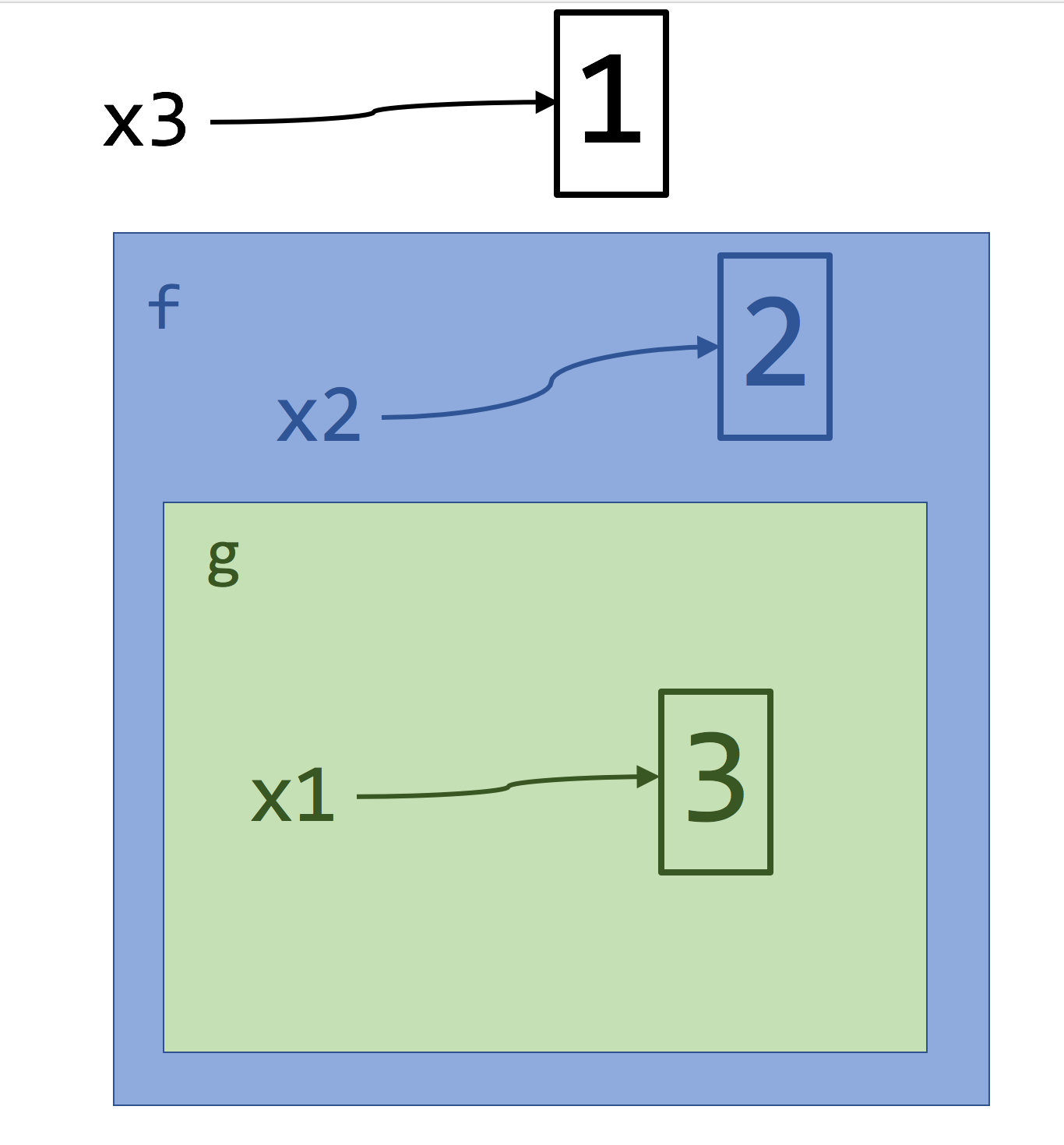
Starting with the inner-most expressions, rename all variables by adding a unique number to all instances of a variable in its scope.
After applying this transformation, it is now safe to use substitution to understand the code. This renaming strategy is known as capture-free capture in lambda calculus. A more precise definition is given on Wikipedia. You can explore the renamed code in codelens and the following figure shows the scope of the rename variables.
(scope_renamed)

One final note. While you are encouraged to think about evaluating expressions using substitution, implementing a language through substitution is inefficient and most languages are implemented with the enviroment model of evalution. Regardless, substitution is still the easiest way to understand evaluation and explains the desire for referentially transparent code.
2.3.5. Evaluation Strategy
When evaluating an expression, we have two choices for the order of evaluation, normal order and applicative order. When evaluating a function call using applicative order, arguments are evaluated first and then the resulting values are substituted into the body of the function. Applicative order evaluation is a form of strict evaluation, where every expression is evaluated as soon as it is encountered. The following sequence of expression represents the step-by-step process of applicative order evaluation.
Applicative Order Evaluation
pow = lambda x, y: x**y
pow(1 + 2, 2*2)
# Evaluate the arguments
pow(3, 4)
# substitute these values in the body
3**4
# Evaluate the body
81
Using codelens, it becomes clear that Python is using strict evaluation, as
x and y are bound to 3 and 4, respectively.
(applicative_order)
Clearly, the function pow is passed 3 and 4, the results of evaluating the
arguments first.
Conversely, function calls that are evaluated using normal order leave the arguments as unevaluated expressions and these expressions are substituted into the body of the function. Using normal order to evaluate functions is a form of lazy evaluation, where we put off the evaluation of arguments as long as possible.
Normal Order Evaluation
pow = lambda x, y: x**y
pow(1 + 2, 2*2)
# Don't evaluate arguments
# Instead substitute in the unevaluated expressions
# into the body of pow
(1+2)**(2*2)
# Now this expression is evaluated using normal order of operation
3**4
If it turns out that the arguments were not used in the function (possible
because of a conditional expression), then we don’t waste time on evaluation.
Consider the following scenario, where cheap is a function that executes
quickly but expensive has a long execution time.
f = lambda x, a, b: a if cond(x) else b
f(x, cheap(x), expensive(x))
When using applicative order, both cheap(x) and expensive(x) will be
evaluated before the body. If it turns out that we didn’t need
expensive(x), we have wasted time. Normal order evaluation will save us the
execution time for expensive(x) when it is not needed. There is always a
trade-off and the trade-off for saving time using lazy evaluation is the
possibility of sapce leaks,
where the build up of unevaluated code can eat more and more memory.
Haskell is an example of a language focused on lazy evaluation, but any language needs some strict evaluation or nothing would ever get done. Similarly, all languages also need some lazy evaluation, in particular conditional expressions and if-else constructions will be evaluated in a lazy fashion in any language. Python uses strict evaluation in function calls, but we will look at other features of Python that allow lazy evaluation in subsequent chapter.
Unfortunately, we won’t be using expressions for all of our programming. In the next section, we will look at some of the statements that are much more convenience when our programs become more complicated.