Comparing Two Population Means: Independent Samples¶

In Chapter 5, we considered inference for a single population mean. Then, in the first part of Chapter 6 we extended these ideas so that comparisons could be made between two groups. Such comparisons were made using differences because the observations in the two groups were related, or dependent.

In this section, we will consider making comparisons between two groups when the observations in one group are independent of the observations in the other group. The methodologies considered here are a bit more involved because it no longer makes sense to simply work with differences. Consider the following example.

Example 6.5: Smoking and Birth Weight¶

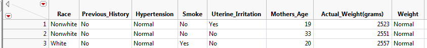
A study was conducted in which the relationship between smoking and birth weights of babies was considered. The data can be found in the file LowBirth.JMP, a portion of which is shown below.

Note

The first observation for a nonsmoker is in NO WAY related to the first observation for a smoker. Therefore, these groups are independent.

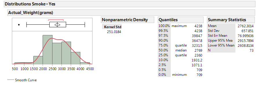
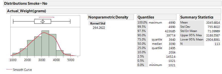
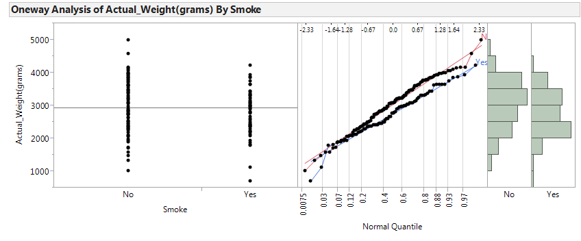
Next, let’s examine birth weight across the two groups: smokers and nonsmokers.

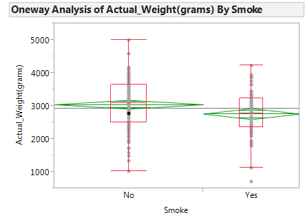
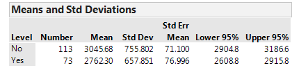
In JMP, we can compare the distributions by selecting Analyze > Fit Y by X. Place the categorical variable (Smoke) in the X, Factor box, and place the numerical variable of interest (Actual_Weight) in the Y, Response box. Select the “Display Options” menu from the red drop-down arrow to display the boxplots and mean diamonds.

Questions:

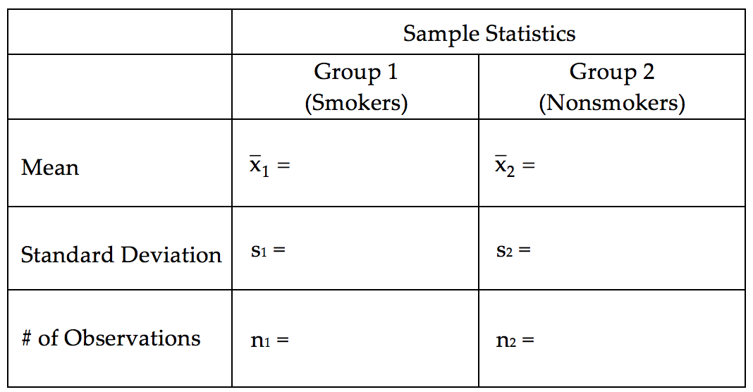
Identify the following sample statistics from the JMP output:

We are interested in the true difference between these two population means. Based on the data, what is your best guess for this difference, and what does it indicate about birth weights for smokers compared to nonsmokers?
If you were to take another sample, is your “best guess” from the previous question likely to change? Explain.

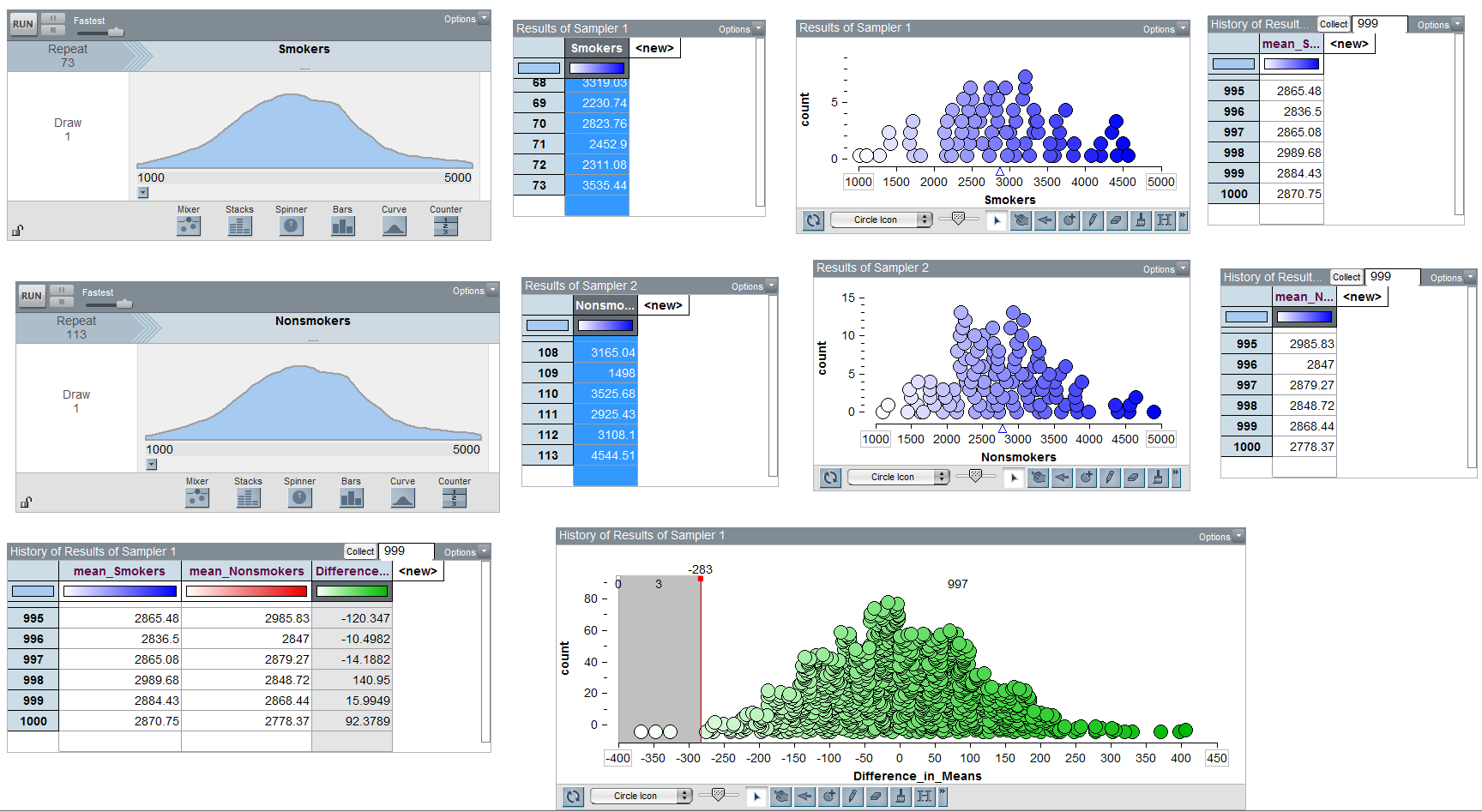
Since the difference will change from sample to sample, in order to make valid inferences about the true population difference, we must first understand how the difference in sample means is expected to change from sample to sample. We start by looking at the bootstrap distribution of the difference in means.

Questions

|image647|

(A) The birth weights were lower, on average, when the mother smoked.
Lower average weights when the mother smoked would result in No - Yes to be positive (i.e. Large - Small).
(B) The birth weights were lower, on average, when the mother did not smoke.
Lower average weights when the mother did not smoke would result in No - Yes to be negative (i.e. Small - Large).
(C) We cannot confidently conclude that the average birth weight was different, when comparing whether or not the mother smoked.
We CAN make a confident conclusion as the interval is all positive.

(A) We are 95% confident that, on average, the babies were between 80.9g and 487.8g heavier for the mothers that smoked.
Remember that positive number, when using No - Yes, indicates a lower average weights when the mother smoked.
(B) We are 95% confident that, on average, the babies were between 80.9g and 487.8g lighter for the mothers that smoked.
Remember that positive number, when using No - Yes, indicates a lower average weights when the mother smoked.
(C) We cannot confidently conclude that the average birth weight was different, let alone the size of the difference.
We CAN make a confident conclusion as the interval is all positive.

Testing a Hypothesis and the Null Distribution¶

If we want to run a formal hypothesis test, we must determine what differences in means are likely to happen by chance when taking random samples from populations with the same mean. The following illustration in Tinkerplots gives us some insight into this.

This should look familiar and remind you of the bootstrap. There is an important difference, in that we need the null distribution to be centered at 0. In the next section, we will look at altering the boostrap distribution to make this the case.

Bootstrap Test for Two Independent Means¶

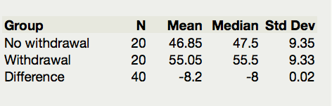
Researchers at Pennsylvania State University investigated whether time perception, a simple indication of a person’s ability to concentrate, is impaired during nicotine withdrawal. Twenty smokers were randomly assigned to a 24-hour smoking abstinence and were asked to estimate how much time had passed during a 45-second period. Another 20 smokers were randomly assigned to a group which was not forced to abstain from nicotine; they were also asked to estimate how much time had passed during a 45-second period. Suppose the resulting data on perceived elapsed time (in seconds) were analyzed as shown below (these results are artificial but are similar to the actual findings). The data can be found in the file Nicotine_all.JMP.

Research Question:

Do those smokers suffering from nicotine withdrawal tend to believe that more time has elapsed than do those not suffering from nicotine withdrawal?

Questions:

(A) The perceived elapsed time for each subject.
The groups (withdrawal or not) are compared on perceived elapsed time, making it the response.
(B) Whether or not the person was suffering from withdrawal.
When comparing groups, the groups label is the explanatory variable.
(C) The average perceived elapsed time for all subjects.
This is a summary method, not a variable.

(A) The perceived elapsed time for each subject.
The groups (withdrawal or not) are compared on perceived elapsed time, making it the response.
(B) Whether or not the person was suffering from withdrawal.
When comparing groups, the groups label is the explanatory variable.
(C) The average perceived elapsed time for all subjects.
This is a summary method, not a variable.

(A) µ_no - µ_with > 0
If withdrawal leads to a larger perceived time, then No - Yes would be negative (i.e. Small - Larger)
(B) µ_no - µ_with < 0
If withdrawal leads to a larger perceived time, then No - Yes would be negative (i.e. Small - Larger)
(C) µ_no - µ_with ≠ 0
We use not-equal when looking for a difference, either way.

(A) Lower/left-tail
If withdrawal leads to a larger perceived time, then No - Yes would be negative (i.e. Small - Larger), so we want to use a lower/left-tail p-value.
(B) Upper/right-tail
If withdrawal leads to a larger perceived time, then No - Yes would be negative (i.e. Small - Larger), so we want to use a lower/left-tail p-value.
(C) Two-tail
Two-tail p-values are for questions that are looking for a difference, either way.

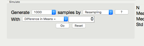
To use the bootstrap distribution to run a hypothesis test, we need to generate the bootstrap distribution then move the distribution so that the mean is centered at the hypothetical mean.

In JMP, we can use the bootstrap to perform a test for the difference in means, by following these steps.

Bootstrap Test in JMP

Save the data somewhere that is easy to access.
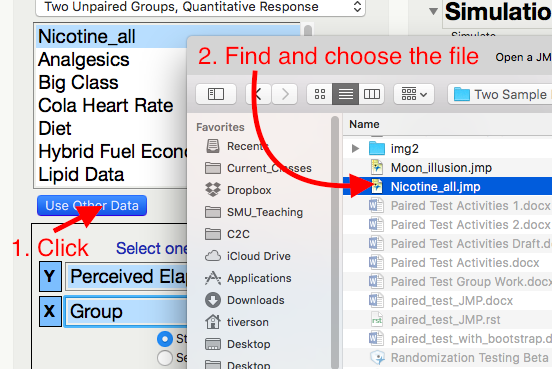
Open the Randomized Test add-in, click Use Other Data, and open the Nicotine_all.jmp data file.
Highlight the Y and X variables.
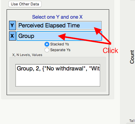
Generate the bootstrap distribution centered at 0. This is due to the fact that we are testing to see if there is a difference between the groups, and consequently the null hypothesis will represent “no difference.”
Note the direction of subtraction on the right hand side. We will need to make sure our alternate hypothesis’s direction matches this subtraction.
At this point we can determine the null and alternative hypothesis, (including the correct order of subtraction.) We do this by considering the research hypothesis in light of the order of subtraction. In this case, the research hypothesis has :math”mu_{with} bigger than \(\mu_{no}\), so \(H_{a}:\mu_{\text{no}} - \mu_{\text{with}} < 0\).
Pick and record the correct p-value for this test.

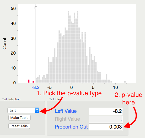
p-value =

Question:

Based on this p-value, write the correct conclusion for this test.

Characteristics of the Sampling Distribution for the Difference in Means¶

The illustration in Tinkerplots helps us understand the intuition behind inference for a difference in means, but we don’t really need Tinkerplots to determine the characteristics of a distribution of differences in means. Instead, we can use what statisticians discovered long ago: as long as the samples are independent, the sampling distribution for the difference in means can be described as follows.

The sampling distribution is centered around \(\mu_1 - \mu_2\).
The standard deviation of our sampling distribution (i.e., standard error) is given as follows:

\[SE_{\bar{x}_1-\bar{x}_2} = \sqrt{\frac{s_1^2}{n_1}+ \frac{s_2^2}{n_2}}\]

The shape of the sampling distribution is approximately normal if (1) both sample sizes are “sufficiently large” OR (2) if both original populations are normally distributed.

Given these characteristics, the test statistic we will use when testing for differences in two population means for INDEPENDENT samples is as follows:

\[t = \frac{(\bar{x}_1 - \bar{x}_2) - (\mu_1 - \mu_2)}{SE_{\bar{x}_1-\bar{x}_2}}\]

This test statistic follows a t-distribution with the following degrees of freedom:

\[df = \frac{\left(\frac{s_1^2}{n_1}+ \frac{s_2^2}{n_2}\right)^2} {\frac{\left(\frac{s_1^2}{n_1}\right)^2}{n_1 - 1}+ \frac{\left(\frac{s_2^2}{n_2}\right)^2}{n_2 - 1}}\]

Therefore, as long as it is reasonable to assume the shape of the distribution of differences in means is approximately normal (see #3 above), we can use the t-distribution to find our p-value. This procedure is typically referred to as the two-sample t-test.

Testing for a Difference in Between Two Unpaired Groups¶

Back to Example 6.5: Carry out the hypothesis test associated with the following research question: Is the average birth weight lower when mothers are classified as smokers?

Step 0: Check the assumptions behind the test to be sure that the t-test is valid.

Are the two groups independent? Explain.
Are both sample sizes sufficiently large? If not, is it reasonable to assume that both populations are normally distributed?

Step 1: Convert the research question into H₀ and H_a.

H₀:

H_a:

Step 2: Calculate the test statistic from your data.

To do this in JMP, click on the red drop-down arrow next to “One-way Analysis...” and select t-test.

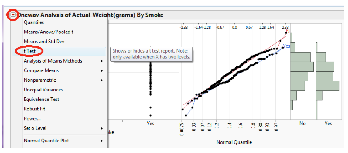
JMP returns the following:

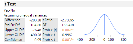
Verify the value of the test statistic in JMP:

\[\begin{split}SE_{\bar{x}_1-\bar{x}_2} = \sqrt{\frac{s_1^2}{n_1}+ \frac{s_2^2}{n_2}}\\ t = \frac{(\bar{x}_1 - \bar{x}_2) - (\mu_1 - \mu_2)}{SE_{\bar{x}_1-\bar{x}_2}}\end{split}\]

Step 3: Determine the p-value.

p-value:

Step 4: Write a conclusion in terms of the original research question.

“We have evidence that the average birth weight is lower when mothers are classified as smokers (p-value = .0038).”

Constructing a Confidence Interval for the Difference in Means¶

Lower Endpoint =

Upper Endpoint =

We often write this confidence interval as:

Interpret the meaning of this 95% confidence interval:

Example 6.6: Time Perception¶

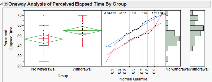
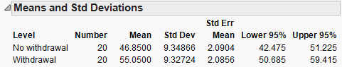
Recall the study conducted by researchers at Pennsylvania State University which investigated whether time perception, a simple indication of a person’s ability to concentrate, is impaired during nicotine withdrawal. This study was discussed in Chapter 5. Twenty smokers were randomly assigned to a 24-hour smoking abstinence and were asked to estimate how much time had passed during a 45-second period. Another 20 smokers were randomly assigned to a group which was not forced to abstain from nicotine; they were also asked to estimate how much time had passed during a 45-second period. Suppose the resulting data on perceived elapsed time (in seconds) were analyzed as shown below (these results are artificial but are similar to the actual findings). The data can be found in the file Nicotine_all.JMP.

Research Question:

Do those smokers suffering from nicotine withdrawal tend to believe that more time has elapsed than do those not suffering from nicotine withdrawal?

Questions:

What is the response variable in this study?
What is the predictor variable in this study?

The data can be summarized using JMP by selecting Analyze > Fit Y by X and placing the predictor (i.e., explanatory) variable in the X, Factor box and the response in the Y, Response box. Then, use the Display Options menu from the red drop-down arrow to add the boxplots and mean diamonds.

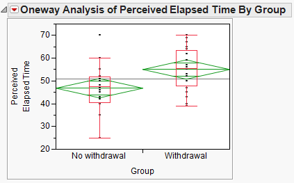
It is clear that the SAMPLE of smokers suffering from nicotine withdrawal has a larger mean perceived elapsed time than those not suffering from withdrawal. However, to determine whether there is a difference in the POPULATION means, we will carry out a hypothesis test.

Step 0: Check the assumptions behind the test to be sure that the test is valid.

Are the two groups independent?

Are both sample sizes sufficiently large? If not, is it reasonable to assume that both populations are normally distributed?

Step 1: Convert the research question into H₀ and H_a

H₀

H_a

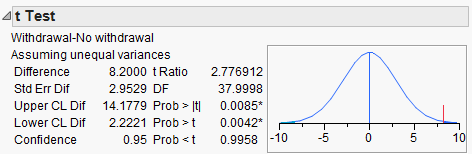
Step 2: Calculate a test statistic from your data.

Verify the value of the test statistic from JMP:

\[\begin{split}SE_{\bar{x}_1-\bar{x}_2} = \sqrt{\frac{s_1^2}{n_1}+ \frac{s_2^2}{n_2}}= \\ t = \frac{(\bar{x}_1 - \bar{x}_2) - (\mu_1 - \mu_2)}{SE_{\bar{x}_1-\bar{x}_2}}=\end{split}\]

Recall that this test statistic comes from a t-distribution w

\[df = \frac{\left(\frac{s_1^2}{n_1}+ \frac{s_2^2}{n_2}\right)^2} {\frac{\left(\frac{s_1^2}{n_1}\right)^2}{n_1 - 1}+ \frac{\left(\frac{s_2^2}{n_2}\right)^2}{n_2 - 1}}=37.9\]

Step 3: Determine the p-value

p-value =

Step 5: Write a conclusion in terms of the original research question.

“The study provides evidence that the average perceived elapsed time is higher for those smokers suffering from nicotine withdrawal than for those not suffering from nicotine withdrawal (p-value = .0042)

Finally, construct a 95% confidence interval for the difference in means:

Lower Endpoint =

Upper Endpoint =

Again, we often write this confidence interval as:

Interpret the meaning of this confidence interval:

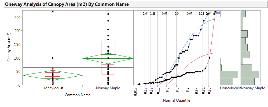
Example 6.7: Tree Canopy Area

Consider the data found in the file NYC_Trees.JMP. Suppose you want to compare the canopy area of the two types of trees. Is the average canopy area of a Honey Locust different from the average canopy area of a Norway Maple? The data are summarized as follows:

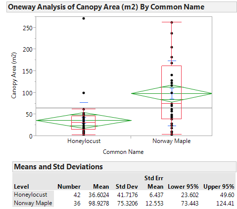
It is clear that the SAMPLE of Norway Maple trees has a higher mean canopy area than the SAMPLE of Honey Locust trees. However, to determine whether the POPULATION mean canopy areas differ between the two groups, we will carry out a hypothesis test.

Step 0: Check the assumptions behind the test to be sure that the test is valid.

Are the two groups independent?

Are both sample sizes sufficiently large? If not, is it reasonable to assume that both populations are normally distributed?

Step 1: Convert the research question into H₀ and H_a

H₀:

H_a:

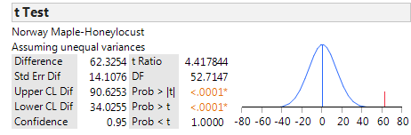
Step 2: Calculate a test statistic from your data.

Step 3: Determine the p-value.

p-value =

Step 4: Write a conclusion in terms of the original research question.

Finally, we can construct a confidence interval for the difference in means:

Lower Endpoint =

Upper Endpoint =

This confidence interval can also be written as:

Interpret the meaning of this 95% confidence interval:

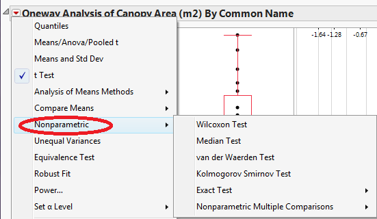
Nonparametric Tests¶

These tests are an alternative to the two-sample t-test for comparing the “average” value of two populations where the samples from each population are taken independently. This test is appropriate when the assumption of normality is violated (as it may have been in the previous example). To obtain the output for these tests, simply select Nonparametric > from the drop-down menu in the upper left-hand corner of the boxplots.

JMP returns the following output when the Wilcoxon Test is selected:

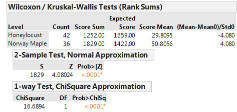
The decision based on Wilcoxon’s test is the same decision that we arrived at using the standard two-sample t-test above. Often, these procedures will agree each other because the above t-test is robust to (i.e. not greatly affected by) departures from normality.

The t-Test for Independent Samples Assuming Equal Variances¶

The two-sample t-test that we discussed in the previous section uses the following test statistic:

\[\begin{split}SE_{\bar{x}_1-\bar{x}_2} = \sqrt{\frac{s_1^2}{n_1}+ \frac{s_2^2}{n_2}}\\ t = \frac{(\bar{x}_1 - \bar{x}_2) - (\mu_1 - \mu_2)}{SE_{\bar{x}_1-\bar{x}_2}}\end{split}\]

Many statisticians use this version of the t-test only when they feel that the variances of the two populations of interest are significantly different from one another (hence it is often called the two-sample t-test assuming unequal variances).

If, however, it is reasonable to assume that the amount of variability in the two populations is about the same, then statisticians often use a slightly different version of the t-test. Assuming the two variances are equal, we can obtain a common estimate of this equal variance (this is called a pooled estimate).

\[SE_{pooled} = \sqrt{\frac{(n_1 - 1)s_1^2 + (n_2 - 1)s_2^2}{(n_1 - 1) + (n_2 - 1)}}\]

Then, the test statistic for the t-test is calculated as follows:

\[t = \frac{(\bar{x}_1 - \bar{x}_2) - (\mu_1 - \mu_2)}{SE_{pooled}}\]

Assuming the two variances are equal, this test statistic comes from a t-distribution with \(df = (n_1 – 1) + (n_2 – 1)\). In practice, the two-sample t-test that was introduced earlier and used throughout the previous section works well, even if the two distributions being compared have the same amount of variability. Therefore, it’s my opinion that instead of worrying about which one to use, just go with the test assuming unequal variances.