Methods for Two Categorical Variables
Example 3.1: MythBusters and the Yawning Experiment
MythBusters, a popular television program on the Discovery Channel, once conducted an experiment to investigate whether or not yawning is contagious. The premise of the experiment was to invite a stranger to sit in a booth for an extended period of time. Fifty subjects were said to be tested in total, of which 34 were “seeded” with a yawn by the person conducting the experiment. The other 16 were not given a yawn seed. Using a two-way mirror and a hidden camera, the experimenters observed and recorded the results which are given below.
| Yawned | Did not Yawn | Total | |
|---|---|---|---|
| Seeded with a yawn | 10 | 24 | 34 |
| Not seeded with a yawn | 4 | 12 | 16 |
Research Hypothesis:
Those “seeded” with a yawn are more likely to actually yawn than those who are not seeded.
When we analyze data on two variables, our first step is to distinguish between the response variable and the explanatory (or predictor) variable.
- Response variable:
- The response variable is the outcome variable on which comparisons are made.
- Explanatory (or Predictor) variable:
- The expanatory variable defines the groups to be compared.
Questions:
- What variables must be measured in the MythBusters Yawning experiment in order to investigate the research hypothesis? Are these variables categorical or numerical?
- Which is the response variable? Which is the explanatory variable?
Descriptive Methods for Two Categorical Variables:
- A contingency table shows the joint frequencies of two categorical variables. The rows of the table denote the categories of the first variable, and the columns denote the categories of the second variable.
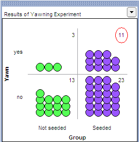
- A mosaic plot gives a visual representation of the relationship between two categorical variables. A mosaic plot graphically presents the information given in the contingency table.
To obtain these descriptive summaries from JMP, the data should be entered as follows:
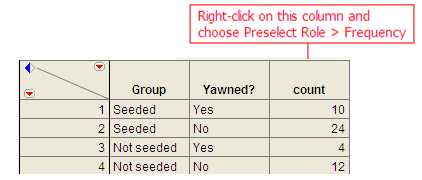
Select Analyze > Fit Y by X. Place the response variable in the Y, Response box and the explanatory variable in the X, Factor box.
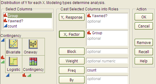
Click OK, and JMP returns the following:
Questions:
- Find the proportion that yawned in the Seeded group.
- Find the proportion that yawned in the Not Seeded group.
- Find the difference in the proportion that yawned between these two groups. Do these proportions differ in the direction conjectured by the researchers?
- Even if the seeding of a yawn had absolutely no effect on whether or not a subject actually yawned, is it possible to have obtained a difference such as this by random chance alone? Explain.
Statistical Inference: Conducting a Simulation Study with Playing Cards
The above descriptive analysis tells us what we have learned about the 50 subjects in the study. Our next goal is to make inferences beyond what happened in the study (i.e., we want to make general statements about the population). Does the higher proportion of yawners in the seeded group provide convincing evidence that being seeded with a yawn actually makes a person more likely to yawn? Note that it is possible that random chance alone could have led to this large of a difference. That is, while it is possible that the yawn seeding had no effect and the MythBusters happened to observe more yawners in the seeded group just by chance, the key question is whether it is probable.
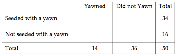
We will answer this question by replicating the experiment over and over again, but in a situation where we know that yawn seeding has no effect (the null model). We’ll start with 14 yawners and 36 non-yawners, and we’ll randomly assign 34 of these 50 subjects to the seeded group and the remaining 16 to the non-seeded group.
Note that we could use playing cards to replicate this experiment: let 14 red cards represent the yawners, and let 36 black cards represent the non-yawners. Shuffle the cards well, and randomly deal out 34 to be the seeded group. This is the first run of our simulation study. Construct the contingency table to show the number of yawners and non-yawners in each group from the first run of our simulation study.
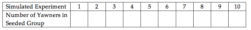
Next, note that if you know the number of yawners in the Seeded group, then you can fill in the rest of the cells in the contingency table. So, for the rest of the simulated runs, we need only keep track of the number of yawners in the Seeded group. Record the number of yawners in the Seeded group from your first simulated experiment in the table below. Then, repeat this randomization process nine more times, recording your results in the table.
Next, create a dotplot of the results:
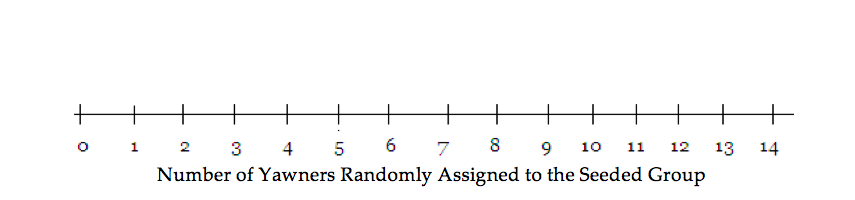
Number of Yawners Randomly Assigned to the Seeded Group
Questions:
- How many randomizations were performed by the class as a whole? What proportion gave results at least as extreme as the actual study (10 or more yawners in the seeded group)?
- Note that the random process used in the simulation study models the situation where the yawn seeding has no effect on whether the subject actually yawns—we simply assume there are 14 people who will yawn no matter what group they are in, and they are assigned to the two groups at random . Based on this simulation study, does it appear that random assignment of yawners to groups will result in 10 or more yawners in the seeded group just by chance? Explain.
- Recall that the MythBusters obtained 10 yawners in the Seeded group. Given your answer to Question 2, would you say that the data provide convincing statistical evidence to support the research question? Explain.
Statistical Inference: Conducting a Simulation Study with Tinkerplots
Note that we could use technology to simulate this process much more efficiently. This will enable us to easily obtain many more simulated results so that we can be more confident in our answer to Question 3 above.
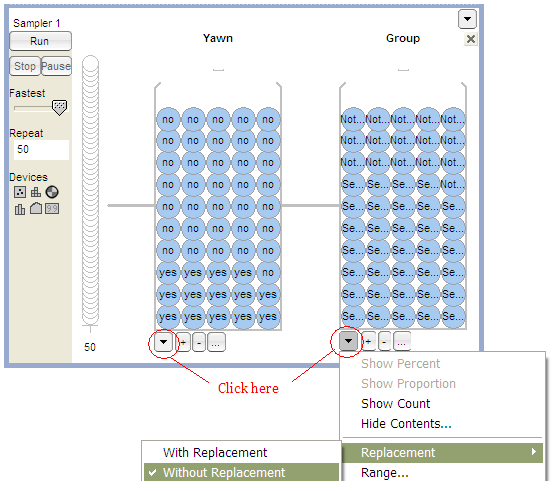
Open the file YawnExperiment.tp from the course website. Note that each mixer contains 50 “subjects.” The first mixer contains 14 yawners and 36 non-yawners; the second mixer contains 34 subjects in the Seeded group and 16 in the Non-seeded group.
Make sure the Repeat value is set to 50 (the number of subjects in the study), and set BOTH mixers to sample Without Replacement (as shown below).
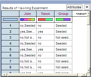
Click Run, and you will see the results of the first simulated trial:
To plot these results, drag a new Plot to the workspace. Drag the predictor variable (Group) to the x-axis and the response variable (Yawn) to the y-axis, as shown below.
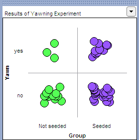
Click on n to count the number in each cell, and you can also vertically stack the dots using the Stack tool.
Note that we are interested in recording the number of yawners in the Seeded group. Place your cursor over this number (circled in red on the below graph), right-click, and choose Collect Statistic. Set the Collect value to 99 in order to obtain a total of 100 simulated results, and click Collect.
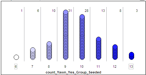
Finally, to graph these outcomes, highlight the “count_Yawn_yes_Group_Seeded” column and drag a new plot into the workspace. Drag a point all the way to the right to organize the dots, and use the Stack tool to vertically stack the dots. Finally, right-click on either endpoint on the x-axis and set “Bin Width” to 1, and use the count tool (n) to count the dots in each bin.
You should see something similar to the following:
Questions:
- What does each dot on the above plot represent?
- What value(s) occurred most often by chance under the null model? Explain why this makes sense.
- How often did we see results at least as extreme as the observed data (10 or more yawners in the seeded group) under the null model? Calculate the proportion of simulated results in which we observed 10 or more yawners in the seeded group. Note that this is an approximate p-value!
- The MythBusters reported the following results: 25% yawned of those not given a yawn seed, and 29% yawned of those given a yawn seed. Then, they cited the “large sample size” and the 4% difference in the proportion that yawned between the seeded and non-seeded group to confidently conclude that yawn seed had a significant effect on the subjects. Therefore, they concluded that the yawn is decisively contagious. Do you agree or disagree with their answer? Justify your reasoning.
Statistical Inference: Fisher’s Exact Test to Obtain Exact p-values
We just used a simulation study to investigate the Mythbusters’ research hypothesis. This is a valid analysis; however, it provides only an approximate p-value. We can obtain the exact p-value using probability theory and a distribution known as the hypergeometric distribution. Details about the hypergeometric distribution are beyond the scope of this course; however, we will discuss Fisher’s Exact Test which uses the hypergeometric distribution to calculate p-values. This is easily carried out in JMP.
Note the output obtained when you used the Analyze > Fit Y by X option:
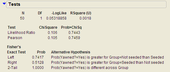
JMP has already used the hypergeometric probability distribution to calculate the probability of observing results at least as extreme as those observed in the MythBusters actual experiment. Now, you can use this output to carry out the test.
Carrying out Fisher’s Exact Test
This test is based on the probability of observing data at least as extreme as the actual observed data. The procedure is carried out as follows.
Example 3.2: Vested Interest and Task Performance
This example is from Investigating Statistical Concepts, Applications, and Methods by Beth Chance and Allan Rossman. 2006. Thomson-Brooks/Cole.*
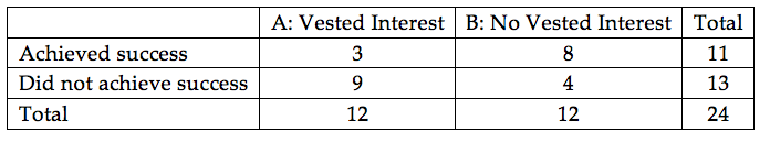
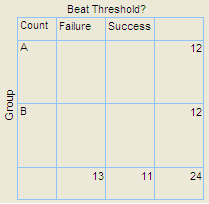
“A study published in the Journal of Personality and Social Psychology (Butler and Baumeister, 1998) investigated a conjecture that having an observer with a vested interest would decrease subjects’ performance on a skill-based task. Subjects were given time to practice playing a video game that required them to navigate an obstacle course as quickly as possible. They were then told to play the game one final time with an observer present. Subjects were randomly assigned to one of two groups. One group (A) was told that the participant and observer would each win $3 if the participant beat a certain threshold time, and the other group (B) was told only that the participant would win the prize if the threshold were beaten. The threshold was chosen to be a time that they beat in 30% of their practice turns. The following results are very similar to those found in the experiment: 3 of the 12 subjects in group A beat the threshold, and 8 of 12 subjects in group B achieved success.”
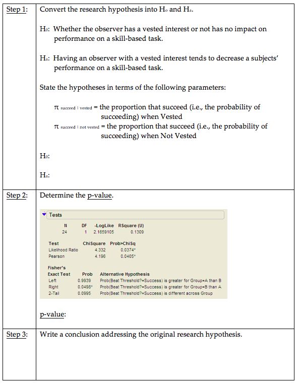
Research Hypothesis:
Having an observer with a vested interest decreases performance on a skill-based task.
Questions:
- What variables must be measured in order to address the research question? Are they categorical or numerical?
- Which is the response variable? Which is the explanatory variable?
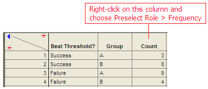
The data can be entered into JMP as follows:
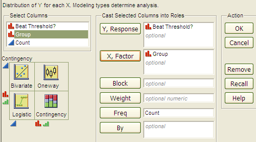
To create the contingency table and the mosaic plot in JMP, select Analyze > Fit Y by X. As always, place the response variable in the Y, Response box and the explanatory variable in the X, Factor box.
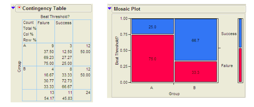
Click OK, and JMP returns the following:
Questions:
- What is the proportion of successes (beating the threshold) for each group?
- What is the difference in the proportion of successes between these two groups? Do these proportions differ in the direction conjectured by the researchers?
- Even if the observer’s interest had absolutely no effect on subjects’ performance, is it possible to have obtained a difference such as this by random chance alone? Explain.
- Next, let’s think about some outcomes that might occur by chance even if having an observer with a vested interest has no real effect on the success rate. We will assume that 11 of the 24 subjects are going to succeed, no matter what group they’re in. Then, we’ll randomly assign them to the two groups of size 12 and see how many of the successes end up in each group purely by chance. Note that this implies that the row and column totals are fixed. What would the counts for the “most extreme” table look like in this case? That is, what possible outcome would give us the most convincing evidence in support of the research hypothesis?
- Give a few more examples of tables that are more extreme than the observed data but not as extreme as the “most extreme” table shown above.
Keep in mind that a p-value is always the probability of seeing results at least as extreme as the observed data. So, JMP uses what is known as the hypergeometric distribution to find the probability of seeing the observed data table and EACH table that is more extreme, assuming that there is no difference in the two groups being compared. The sum of these probabilities is the p-value from Fisher’s exact test.
Fisher’s Exact Test to Obtain Exact p-values
Example 3.3: Claritin and Nervousness
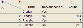
An advertisement by the Schering Corporation in 1999 for the allergy drug Claritin mentioned that in a pediatric randomized clinical trial, symptoms of nervousness were shown by 4 of 188 patients on Claritin and 2 of 262 patients taking a placebo.
Research Hypothesis:
The proportion who experience nervousness is greater for those who take Claritin than for those who take the placebo.
The data can be found in the file Claritin.JMP.
Questions:
- What variables must be measured in order to address the research hypothesis?
- Which is the response variable? Which is the explanatory variable?
- Fill in the following contingency table based on the data table from JMP.
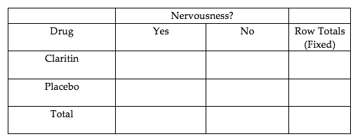
- Find the proportion that experience nervousness in each group.
Next, use JMP to carry out Fisher’s Exact Test for these data.
Observational Studies vs. Designed Experiments
Reconsider the “Vested Interest and Task Performance” example. Fisher’s exact test provided evidence that the proportion of successes was in fact smaller for the vested interest group (p-value = .0498). Now, the question is this: can we conclude that having a vested interest really is the cause of the decreased performance?
The answer to this question lies in whether the experiment itself was a designed experiment or an observational study.
- Observational Study
- An *observational study* involves collecting and analyzing data without randomly assigning treatments to experimental units.
- Designed Experiment
- On the other hand, in a *designed experiment*, a treatment is randomly imposed on individual subjects in order to observe whether the treatment causes a change in the response.
Key statistical idea:
The random assignment of treatments used by researchers in a designed experiment should balance out between the treatment groups any other factors that might be related to the response variable. Therefore, designed experiments can be used to establish a cause-and-effect relationship (as long as the p-value is small).
On the other hand, observational studies establish only that an association exists between the predictor and response variable. With observational studies, it is always possible that there are other lurking variables not controlled for in the study that may be impacting the response. Since we can’t be certain these other factors are balanced out between treatment groups, it is possible that these other factors could explain the difference between treatment groups.
Note that the “Vested Interest and Task Performance” study is an example of a designed experiment since participants were randomly assigned to the two groups. We were trying to show that having a vested interest caused a decreased task performance. The small p-value rules out observing the decreased performance in the vested interest group simply by chance, and the randomization of subjects to treatment groups should have balanced out any other factors that might explain the difference. So, the most likely explanation left is that having a vested interest really is the cause of the decreased task performance.
Example 3.4: Alcoholism and Depression
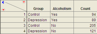
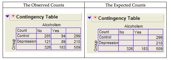
Past research has suggested a high rate of alcoholism in families of patients with primary unipolar depression. A study of 210 families of females with primary unipolar depression found that 89 had alcoholism present. A set of 299 control families found 94 present.
Research Hypothesis:
The proportion of families afflicted by alcoholism differs depending on whether or not the female in the family had primary unipolar depression.
The data can be found in the file Depression.JMP:
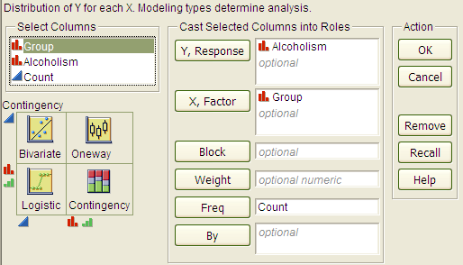
To analyze these data, choose Analyze > Fit Y by X.
Questions:
- Which is the response variable?
- Which is the explanatory variable?
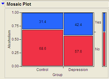
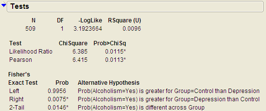
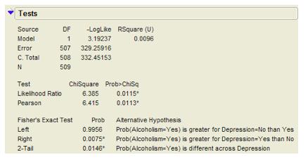
The JMP output is shown below:
Questions:
- Identify the proportion of families with alcoholism in both groups.
- Is there evidence that the proportion of families afflicted by alcoholism differs depending on whether or not the female in the family had primary unipolar depression? Use the JMP output to answer this question.
- Can we say that a female having unipolar depression causes alcoholism in her family? Explain your reasoning.
Chi-Square Test (Alternative to Fisher’s Exact Test)
Fisher’s exact test from the previous section can be used for either upper-tailed, lower-tailed, or two-tailed hypothesis tests for differences in two proportions. The Chi-square test is another procedure we can use to test for differences between two proportions. However, this procedure can be used for ONLY TWO-SIDED TESTS! Consider the data from Example 4.4.
H0: The proportion of families afflicted by alcoholism is the same regardless of whether ornot the female in the family suffers from primary unipolar depression.Ha: The proportion of families afflicted by alcoholism differs depending on whether or notthe female in the family suffers from primary unipolar depression.
With the chi-square test, the evidence from our sample will consist of a test statistic, which for this test is given as follows:
Question:
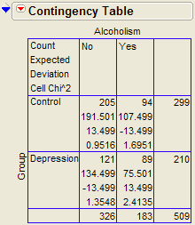
Where do we get the expected counts?
We can also use JMP to calculate the expected counts, deviances, and cell contributions to find the test statistic:
Questions:
- What does it mean when the test statistic is “large”?
- At what point does the test statistic provide evidence to support our research question?
Find the p-value:
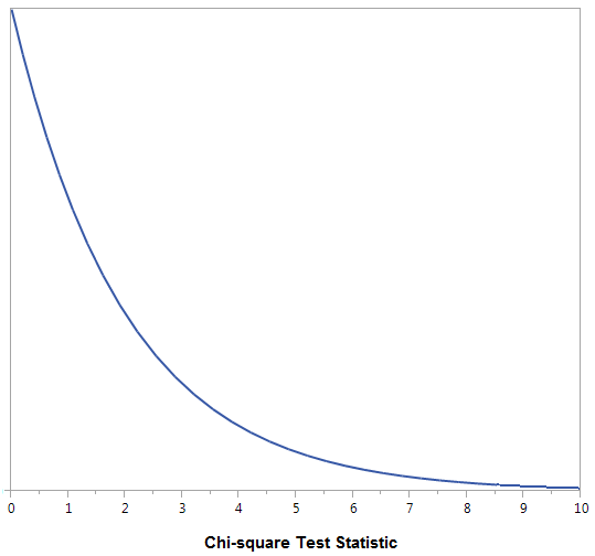
Recall that the Chi-Square test uses a distribution known as the chi-square (χ:sup:2) distribution. The chi-square distribution takes on only positive numbers and is a continuous distribution. In addition, this distribution is indexed by its degrees of freedom (or df). For this test, this is given by df = (r - 1)(c - 1). When the null hypothesis is true, the test-statistic follows the chi-square distribution with df = (r - 1)(c - 1). .
The following graph shows the chi-square distribution with df = 1. The p-value is found by plotting the chi-square test statistic on the x-axis and calculating the area under the curve above the test statistic.
Note that the output for the chi-square test automatically appears when you select Analyze > Fit Y by X.
Assumptions behind the Chi-Square Test:
The chi-square test for independence may be inappropriate for tables with very small expected cell frequencies. One rule of thumb suggests that most of the expected cell frequencies in the table should be 5 or more; otherwise, the chi-square approximation may not be reliable. JMP and most other statistical software packages will warn you when the results of the chi-square test are suspect.
Also, each observation in the study can be classified into only one cell of the contingency table, and the observations must be independent.
Example 3.5: Mice and Tobacco Smoke
Ten mice (6–8 weeks old) were randomly assigned to one of two groups; five were exposed to simulated environmental tobacco smoke for 6 h/day, 5 days/week for 5 months. The other 5 mice were kept in clean air during this time period. Then, all of the mice were allowed to recover for a further 4 months in filtered air before being killed for analysis of lung tumor incidence. The results are shown below.
| Tumor | No tumor | |
|---|---|---|
| Treated | 5 | 0 |
| Control | 2 | 3 |
Research hypothesis:
The proportion of mice that develop a lung tumor differs between those exposed to tobacco smoke and the control group.
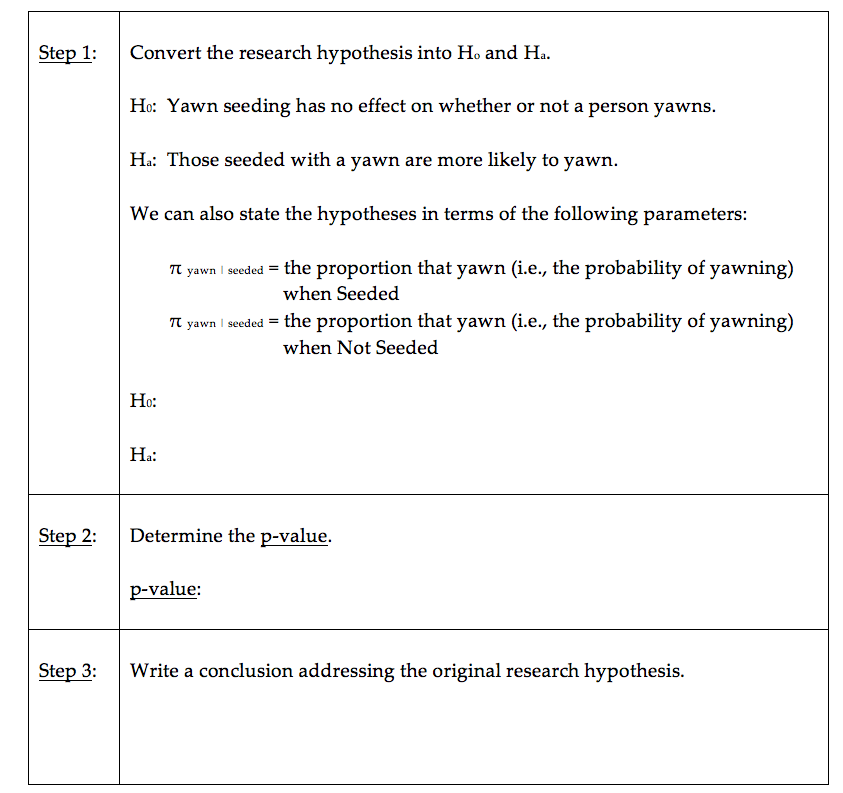
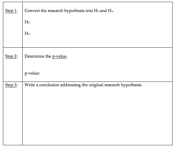
Step 1: Convert the Research Hypothesis into H:sub:`o` and H:sub:`a`.
H0: The proportion of mice that develop a lung tumor when exposed to tobacco does not differ from the proportion that develop a lung tumor when not exposed to tobacco.
Ha: The proportion of mice that develop a lung tumor differs between those exposed to tobacco smoke and those not exposed.
Equivalently, we can state the hypotheses as follows:
H0:
Ha:
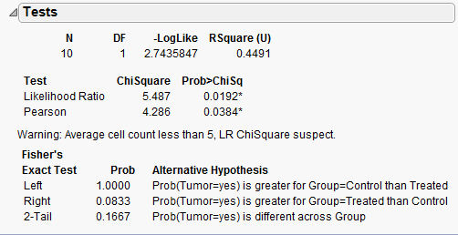
Step 2: Find the p-value for the data.
p-value from Fisher’s exact test: _____________
p-value from Chi-Square test: _____________
Keep the assumptions behind the chi-square test in mind:
The chi-square test for independence may be inappropriate for tables with very small expected cell frequencies. One rule of thumb suggests that most of the expected cell frequencies in the table should be 5 or more; otherwise, the chi-square approximation may not be reliable.
Also, each observation in the study can be classified into only one cell of the contingency table, and the observations must be independent.
Questions:
- Do the assumptions behind the chi-square test appear to be met? Explain.
- Which test should we use – Fisher’s exact or Chi-square? Explain.
Step 3: Write a conclusion addressing the original research hypothesis.
Confidence Interval for the Difference in Proportions
Recall our conclusion from Example 3.4 after conducting a hypothesis test: “We have evidence the proportion of families afflicted by alcoholism differs depending on whether or not the female in the family had primary unipolar depression.” The next natural question is as follows: how large is the difference in these proportions?
We can start by finding the difference in these proportions obtained from the sample:
- \hat{\pi}_{\mathrm{Alcoholism|Depression}} =
- \hat{\pi}_{\mathrm{Alcoholism|Control}} =
- \hat{\pi}_{\mathrm{Alcoholism|Depression}} - \hat{\pi}_{\mathrm{Alcoholism|Control}} =
Task
Interpret this difference in the sample proportions:
Next, note that when discussing the results of the Alcoholism and Depression example, we want to make conclusions that allow us to compare the alcoholism rate in the POPULATION of families of all females affected by depression versus those who are not. The difference we just calculated describes the size of the difference in the proportions obtained in our SAMPLE. To generalize these results to the population, we must calculate a confidence interval for the risk difference.
To find the confidence interval of interest for the previous example, we need the following.
Let \hat{\pi}_1 = \hat{\pi}_{\mathrm{Alcoholism\,Depression}} and \hat{\pi}_2 = \hat{\pi}_{\mathrm{Alcoholism\|Control}} .
An ESTIMATE of the difference in the two proportions (i.e., the risk difference):
\[\hat{\pi}_1 - \hat{\pi}_2\]An appropriate QUANTILE:
This confidence interval requires quantiles from the standard normal distribution which will vary depending on the level of confidence.
Level of Confidence 90% 95% 99% z-Quantile 1.645 1.96 2.58 For a 95% confidence interval, z-Quantile =
The STANDARD DEVIATION OF THE ESTIMATE (i.e., the standard error):
The standard deviation of the difference between two proportions is calculated as follows.
\[\sqrt{\frac{\hat{\pi}_1(1-\hat{\pi}_1)}{n_1} +\frac{\hat{\pi}_2(1-\hat{\pi}_2)}{n_2}}\]
The 95% confidence interval for the risk difference is then calculated as follows:
\[\hat{\pi}_1 - \hat{\pi}_2 \pm 1.96\sqrt{\frac{\hat{\pi}_1(1-\hat{\pi}_1)}{n_1} +\frac{\hat{\pi}_2(1-\hat{\pi}_2)}{n_2}}\]
Note that we could have also reversed the order of the proportions when finding the difference:
\[\hat{\pi}_2 - \hat{\pi}_1 = \hat{\pi}_{\mathrm{Alcoholism|Control}} - \hat{\pi}_{\mathrm{Alcoholism|Depression}}\]
The 95% confidence interval for the risk difference is then calculated as follows:
\[\hat{\pi}_2 - \hat{\pi}_1 \pm 1.96\sqrt{\frac{\hat{\pi}_1(1-\hat{\pi}_1)}{n_1} +\frac{\hat{\pi}_2(1-\hat{\pi}_2)}{n_2}}\]
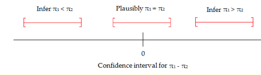
Guidelines for Interpreting a Confidence Interval for a Difference in Proportions:
- Check whether zero falls in the interval or not. If it does, it is plausible (but not proof!) that the two proportions are equal.
- If all values in a 95% confidence interval for \pi_1 - \pi_2 are positive, then you can infer that \pi_1 > \pi_2 interval tells you how much bigger (with 95% certainty) \pi_1 is. Similarly, if all values in a confidence interval for \pi_1 - \pi_2 are negative, then you can infer that \pi_1 < \pi_2. The interval tells you how much bigger \pi_2 is.
Questions:
- Interpret the 95% confidence interval for the difference in proportions in this problem.
- Does this confidence interval agree with the results of the hypothesis test? Explain.
Example 3.6: Gender and Health Insurance
In 2010, the U.S. Congress passed the historic health care reform bill that will provide some type of coverage for the 32 million Americans currently without health care insurance. Prior to this, several studies were carried out to investigate how widespread the lack of medical coverage really was and to determine which segments of the population were most at risk. One such study compared the proportion of uninsured across gender using data from the U.S. Census Bureau Current Population Survey, and the results are shown below.
| Uninsured | Insured | Total | |
|---|---|---|---|
| Female | 21,131 | 132,257 | 153,388 |
| Male | 25,208 | 122,886 | 148,094 |
Questions:
- Find the proportion of females that are uninsured.
- Find the proportion of males that are uninsured.
- Find the difference in the sample proportions.
- Find a 95% confidence interval for this difference.
- Interpret the confidence interval from the previous question.
Example 3.7: Adoption and Suicide Attempts
In September of 2013, researchers from the University of Minnesota published a study in the journal Pediatrics. This study was described in a Fox News article titled “Adopted teens may be at higher risk of suicide.” This article described the results as follows:
[The researchers] examined data from an existing University of Minnesota study of 692 adopted children and 540 non-adopted siblings in Minnesota… All of the adopted kids, who were between 11 and 21 years old during the study period, had been taken in by their families before age two. Almost three quarters of the adopted children were born abroad, most of the foreign-born children were from South Korea and 60 percent of those were girls. At the beginning of the study, and again about three years later, the researchers asked participating families if the children had made a suicide attempt. Over the three years of the study, 56 children attempted suicide at least once, according to the family members’ reports. Of those kids, 47 were adopted and nine were not adopted.
Questions:
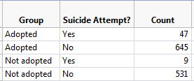
- Create a table of counts based on the data obtained in this study:
| Suicide Attempt | No Suicide Attempt | Totals | |
|---|---|---|---|
| Adopted | |||
| Not adopted | |||
| Totals |
- Find the proportion of adopted children that attempted suicide.
- Find the proportion of non-adopted children that attempted suicide.
- Find and interpret a 95% confidence interval for the difference in proportions.
Calculating Risks and the Relative Risk
The confidence interval calculated above helps us to quantify the discrepancy in the proportion of adopted versus non-adopted that had attempted suicide. We could also measure the amount of discrepancy between these two proportions based on something called relative risk. This involves taking the ratio of the two proportions instead of the difference.
Note that in the previous example, our estimate of the proportion of adopted children that had attempted suicide could be viewed as an estimate of the probability of an adopted child attempting suicide (the same could be said for the non-adopted group). When we calculate the probability of an adverse event, we sometimes refer to this probability as a risk.
For example, we can calculate the risk of attempting suicide for both groups in this study as follows:
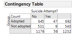
| Suicide Attempt | No Suicide Attempt | Total | |
|---|---|---|---|
| Adopted | 47 | 645 | 692 |
| Not adopted | 9 | 531 | 540 |
- Risk of attempting suicide for the Adopted group =
- Risk of attempting suicide for the Not Adopted group =
The relative risk (also called the risk ratio) is then computed as follows:
Note
We interpret this number by saying that in this study, the risk of suicide attempt for adopted children was ______ times as large as the risk of suicide attempt for children who were not adopted. In other words, adopted children were ______ times as likely to attempt suicide as were non-adopted children.
A relative risk value of 1.0 is the reference value for making comparisons. That is, a relative risk of 1.0 says that there is no difference in the two proportions of interest.
When you are interpreting a relative risk, you MUST consider which value you have in the numerator. For example, we could have also calculated the relative risk as follows:
\[\mathrm{Relative\,Risk} = \frac{\hat{\pi}_{\mathrm{Suicide|Not\,Adopted}}}{\hat{\pi}_{\mathrm{Suicide|Adopted}}}\]How would we interpret this value?
Calculating Odds and the Odds Ratio
Another quantity that is often used to describe differences in categorical outcomes between groups is the odds ratio. This ratio is used more commonly in practice than the relative risk ratio; however, it is more difficult to interpret and is sometimes harder to understand.
Before computing an odds ratio, we first need to compute the odds for both groups:
- Odds
- Consider our Adoption and Suicide Attempt example. For each group (Adopted and Not Adopted), the odds of attempting suicide is computed as the number of subjects in that group that attempted suicide divided by the number in that group that did not attempt suicide.
Recall the contingency table for this example.
| Suicide Attempt | No Suicide Attempt | Total | |
|---|---|---|---|
| Adopted | 47 | 645 | 692 |
| Not adopted | 9 | 531 | 540 |
Find the odds of attempting suicide for both groups:
- Odds of Attempting Suicide in the Adopted Group:
- Odds of Attempting Suicide in the Non-adopted Group:
The odds ratio is then simply the ratio of the odds for the two groups:
We interpret this quantity by saying that in this study, the odds of attempting suicide were about ________ times as high for adopted children as for non-adopted children.
We could also have calculated the odds ratio as follows:
How would we interpret this value?
Example 3.8: Smoking and Lung Cancer
The data in the contingency table shown below are the results of a case-control study published back in 1950 (this was one of the first studies linking smoking to lung cancer). Note that in this study, the researchers found one control subject for every case of lung cancer in their study.
Source:
Doll and Hill, British Medical Journal, 1950, p. 739-748.
| Cases (Had Lung Cancer) | Controls (No Lung Cancer) | Total | |
|---|---|---|---|
| Smoked | 688 | 650 | 1338 |
| Never Smoked | 21 | 59 | 80 |
| Total | 709 | 709 | 1418 |
Questions:
- Even though it is not appropriate to calculate relative risk of having lung cancer with this case-control study, do this for illustrative purposes only.
- Calculate the odds ratio for having lung cancer.
Now, suppose that the researchers had found two control subjects for every case and that the results were as shown below.
| Cases (Had Lung Cancer) | Controls (No Lung Cancer) | Total | |
|---|---|---|---|
| Smoked | 688 | 1300 | 1988 |
| Never Smoked | 21 | 118 | 139 |
| Total | 709 | 1418 | 2127 |
Questions:
- Once again, calculate the relative risk of having lung cancer with this case-control study, even though it is not appropriate.
- Compare your answers to Questions 1 and 3 from above and use them to explain why it is not appropriate to calculate relative risk with case-control studies.
- Calculate the odds ratio for having lung cancer. How does this answer compare to your answer to Question 2 from above?
Example 3.9: When is the Relative Risk Close to the Odds Ratio?
Consider the following hypothetical example comparing survival rates between two groups.
| Survived | Died | Total | |
|---|---|---|---|
| Group A | 98 | 2 | 100 |
| Group B | 99 | 1 | 100 |
Questions:
- Compute the relative risk of death.
- Compute the odds ratio for death.
- What do you notice about the overall probability of death? In this case, how close are the relative risk and the odds ratios?
Now, suppose the results were as shown below, instead.
| Survived | Died | Total | |
|---|---|---|---|
| Group A | 25 | 75 | 100 |
| Group B | 75 | 25 | 100 |
Questions:
- Compute the relative risk of death.
- Compute the odds ratio for death.
- What do you notice about the overall probability of death? In this case, how close are the relative risk and the odds ratios?
Relative Risk and Odds Ratios in JMP
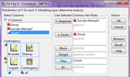
To discuss the calculation of the relative risk and the odds ratio in JMP, let’s once again consider the Adoption and Suicide Attempt example. The data should be entered in JMP as follows.
In JMP, select Analyze > Fit Y by X and enter the following:
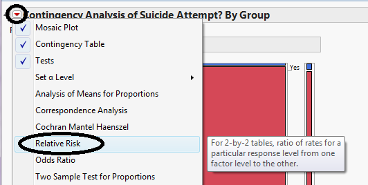
Click OK. On the output that appears, click on the red drop-down arrow next to Contingency Analysis… and select Relative Risk.
Enter the following and click OK.
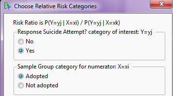
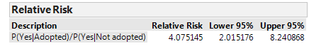
JMP returns the following:
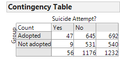
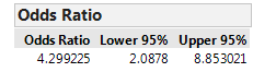
If you also ask for the Odds Ratio from this red drop-down arrow, JMP returns this quantity:
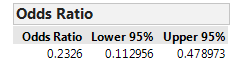
Note that JMP is by default computing the odds of NOT attempting suicide since this column appears first in the contingency table. It is then computing the odds ratio with the Adopted Group in the numerator, since this row appears first in the table.
After re-ordering the columns for the Suicide Attempt? variable we obtain the following:
Questions:
- Verify that the relative risk and odds ratio shown match our calculations.
- Note that JMP gives a confidence interval for both the relative risk and the odds ratio. What would it imply if either of these confidence intervals was to include the value one? Explain.
Example 3.10: Importance of Considering Absolute Risk
In 1995, the UK Committee on Safety of Medicines issued a warning that birth control pills increased the risk of life-threating blood clots. The data on which these conclusions were drawn were very similar to the following outcomes.
| Birth Control Pill? | Blood Clot | No Blood Clot | Total |
|---|---|---|---|
| Yes | 2 | 6998 | 7000 |
| No | 1 | 6999 | 7000 |
| Total | 3 | 13,997 | 14,000 |
Questions:
- Find the risk of blood clots for those using birth control pills.
- Find the risk of blood clots for those not using birth control pills.
- Find and interpret the relative risk.
- All of the headlines related to this study mentioned the “two-fold risk increase” or “100% risk increase” in blood clots because of the birth control pill. What do you suppose happened to the number of birth control users after these results were publicized? Are there any potential negative consequences to this? Explain.
- What do you suppose would have happened had patients also considered the absolute risk of blood clots for those using birth control pills?
Inferences for Comparing Two or More Proportions - Chi-Square Test of Independence
In this section, we will once again discuss a hypothesis testing procedure that uses the chi-square distribution. Specifically, this is known as the Chi-Square Test of Independence.
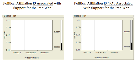
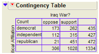
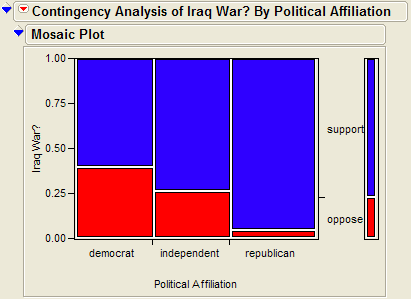
Example 3.11: Support for Iraq War and Political Affiliation
In March of 2003, the Pew Internet & American Life Project commissioned Princeton Survey Research Associates to develop and carry out a survey of what Americans thought about the recent war in Iraq. Some of the results of this survey of over 1,400 American adults are given in the JMP data file IraqWar.JMP. (Source: McClave & Sincich, Problem 13.33) Responses to the following questions were recorded:
- Do you support or oppose the Iraq War?
- Do you ever go online to access the Internet or World Wide Web?
- Do you consider yourself a Republican, Democrat, or Independent?
- In general, would you describe your political views as very conservative, conservative, moderate, liberal, or very liberal?
- What is your race?
- Do you live in a suburban, rural, or urban community?
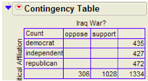
Note that this investigation requires us to focus on only two of the measured variables: Support for the Iraq War and Political Affiliation. First, let’s summarize the data using JMP. Select Analyze > Fit Y by X and enter the following:
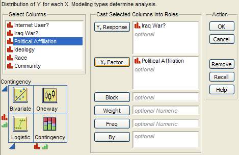
JMP returns the contingency table and mosaic plot:
Questions:
- What can you say about the association between Support for the Iraq
War and Political Affiliation based on the data obtained in the sample?
On the graphs below, sketch hypothetical examples of each of the following situations.
Carrying out the chi-square test of independence:
Assumptions behind the Chi-square Test:
The chi-square test of independence may be inappropriate for tables with very small expected cell frequencies. One rule of thumb suggests that most of the expected cell frequencies in the table should be 5 or more; otherwise, the chi-square approximation may not be reliable. Also, all observations that are counted in the contingency table should be independent of each other.
Step 1: Convert the research question into H_0 and H_a:
Ho:
Ha:
Step 2: Calculate a test statistic and p-value from the data.
Observed counts:
Finding the expected counts:
Once we have the expected counts, we can calculate the test statistic as follows:
Questions:
- What does it mean when the test statistic is “large”?
- At what point does the test statistic provide evidence to support our research question?
Finding the p-value:
The Chi-Square test uses a distribution known as the chi-square \chi^2 distribution. The chi-square distribution takes on only positive numbers and is a continuous distribution. In addition, this distribution is indexed by its degrees of freedom (or df). For this test, this is given by
You can use the following function in EXCEL to find the p-value: =CHIDIST(test statistic, df).
The following graph shows the chi-square distribution with df = 2. The p-value is found by plotting the chi-square test statistic on the x-axis and calculating the area under the curve above the test statistic.
The output for the chi-square test is also given in the JMP output:

Step 3: Write a conclusion in the context of the problem
Finally, since we have determined that there is a significant association between support for the Iraq war and political affiliation, we can describe this relationship based on the patterns displayed in the mosaic plot.
Chi-square Test of Independence versus Chi-square Test of Homogeneity
In the context of our Iraq War example, some statisticians might differentiate between these two versions of the chi-square test as follows.
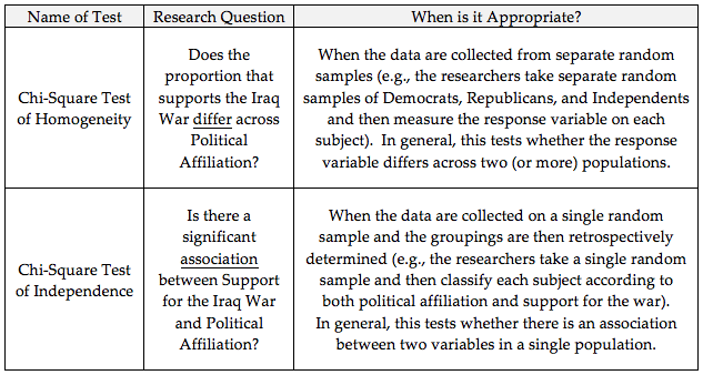
Note that the choice of homogeneity versus independence depends on only the study design and that the phrasing of the research question is slightly different between the two versions. The actual study described here in Example 3.11 involved a single random sample, so this is technically a chi-square test of independence. If the researchers had taken separate random samples of U.S. citizens from each political affiliation group, how would our results have changed? The answer is… not much. We would have calculated the chi-square test statistic in the same way, so we would have obtained the same test statistic and the same p-value. Our conclusion might have focused on there being a significant difference in the proportion that supports the war across political affiliation instead of focusing on there being a significant relationship between the two variables, but the overall story would have remained the same.
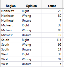
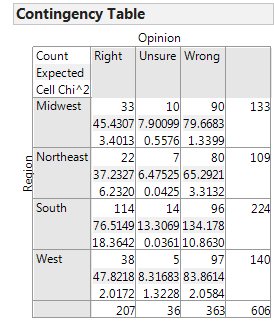
Example 3.12: Opinions on Disciplining Children across Regions of U.S.
On September 16-17, 2014, an NBC News/Marist Poll surveyed a random sample of 606 adults nationwide. Respondents were asked the following question: “Do you think it is right or wrong for parents to discipline their children by striking them - either with a paddle, switch, or belt?”
The results were separated according to the Region of the U.S. in which the respondent lived (Northeast, Midwest, South, or West). The data are summarized in the following table.
| Right | Wrong | Unsure | Totals | |
|---|---|---|---|---|
| Northeast | 22 | 80 | 7 | 109 |
| Midwest | 33 | 90 | 10 | 133 |
| South | 114 | 96 | 14 | 224 |
| West | 38 | 97 | 5 | 140 |
| Totals | 207 | 363 | 36 | 606 |
Research Question:
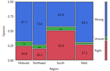
Is there a statistically significant association between Region and Opinion on this Discipline Issue?
First, since we don’t have access to the raw data, we can enter the data from the contingency table into JMP as follows (see the file Discipline.jmp posted on the course website).
We can then use the Analyze > Fit Y by X menu to obtain the desired output:
Step 1: Convert the research question into H_0 and H_a:
Ho:
Ha:
Step 2: Find the test statistic and p-value from the data.
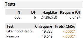
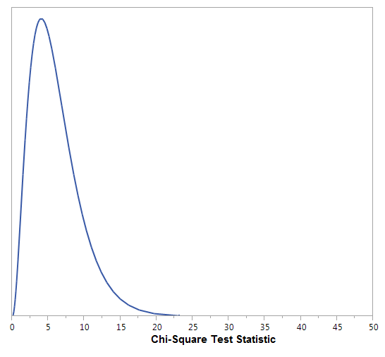
Note
The chi-square distribution with df = 6 is shown below. Do you see why the p-value is so small?
Step 3: Write a conclusion in the context of the problem.
Finally, note that if we determine a significant relationship exists between the two variables of interest, we should take the time to describe this relationship.
Also, we can look at each cell’s contribution to the test statistic to informally determine what is driving the significance of this relationship:
Comments: