6. Methods for a Single Categorical Variable
6.1. Formal Hypothesis Tests With Simulations
The general approach used in a statistical investigation is shown in the following diagram. Note that every investigation starts with a question that gets converted to a research hypothesis. Though we will rarely design our own studies in this course, we will discuss good strategies and best practices for collecting data throughout the semester. Most of our attention will be devoted to descriptive and inferential methods for analyzing the data, how we decide whether the data supports the research question, and how to write conclusions that appropriately summarize the results of the study.
| A Statistical Investigation |
|---|
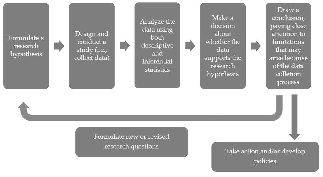 |
In Chapter 2, we will discuss methods for making decisions concerning research hypotheses involving only a single categorical variable. Even though we’ll be adding lots of terminology and formalities along the way, we will use the same logical approach to investigating research questions that was introduced in Chapter 1.
6.1.1. Formal Hypothesis Testing
You are most likely already familiar with several methods for descriptive statistics (e.g., calculating percentages, constructing bar charts or pie charts, etc.). Inferential methods, however, may be new to you. Again, inferential statistics involves drawing conclusions about the larger population that our sample was supposed to represent. In several examples introduced in Chapter 1, we used a logical process to make statistical decisions concerning a population of interest – we were actually using inferential statistics already! Now, we will add more structure to these statistical investigations by introducing an inferential statistics procedure known as hypothesis testing. Note that in this chapter, we look at hypothesis testing for only research questions involving a single categorical variable. Before we discuss this procedure, however, we must introduce a few more definitions.
- Hypothesis Testing
- Hypothesis testing is a procedure, based on sample evidence and probability, used to test a claim regarding a population parameter. The test will measure how well our observed sample statistic agrees with some assumption about this population parameter.
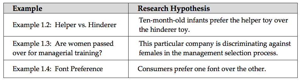
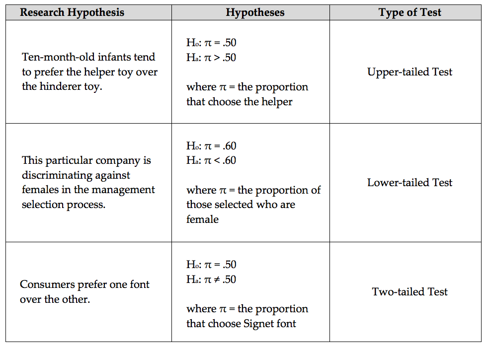
Before you begin a hypothesis test, you should clearly state your research hypothesis. For instance, let’s reconsider the research hypotheses from three of our previous examples.
Once the research hypothesis has been developed, we typically formulate what are known as the null and alternative hypotheses. The null and alternative hypotheses are both statements about the parameter of interest in the study.
6.1.2. The Null and Alternative Hypotheses
Setting Up the Null and Alternative Hypothesis
- The null hypothesis, Ho, is what we will assume to be true (i.e., we will assume for the time being that whatever effect we want to detect doesn’t exist in reality). We will then evaluate the observed outcome from our study against what outcomes we expected to see under the null hypothesis. This will always contain a statement saying that the population parameter is equal to some value.
- The alternative hypothesis, Ha, is what we are trying to show. Therefore, the research hypothesis is simply restated here as if it were true in the alternative hypothesis. This will always contain statements of inequality, saying that the population parameter is less than, greater than, or different from the value in the null hypothesis.
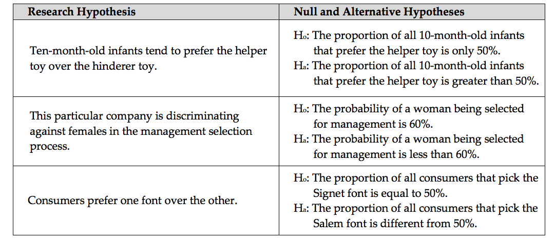
For our three examples, the null and alternative hypotheses are shown below.
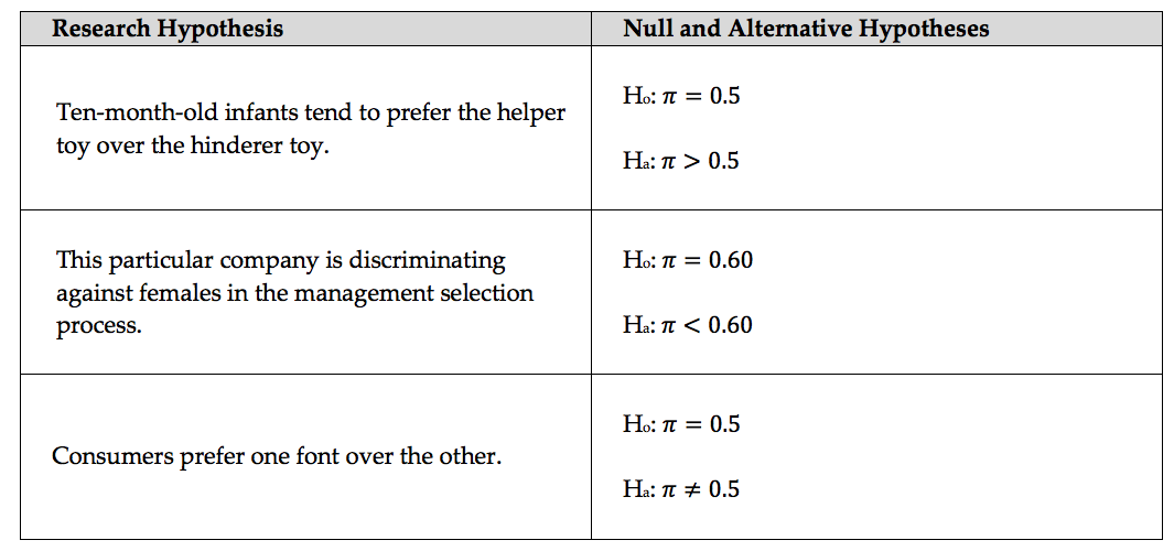
Note that we can also state these hypotheses in terms of the population parameter of interest using formal notation:
6.1.3. What Constitutes Strong Evidence?
6.1.4. Evaluating Evidence Using P-Values
In each of our three examples, we essentially assumed the null hypothesis was true when setting up our spinner for the Tinkerplots investigation. Then, we used the results simulated under this scenario to help us decide whether observing results such as our sample data would be an unusual event if the null hypothesis were true.
Up to this point, whether an observed study result was considered unusual (or extreme) has been a rather subjective decision. Now, we will discuss the guidelines used by statisticians to determine whether an observed study result is extreme enough under the null hypothesis for us to conclude that the evidence supports the research hypothesis.
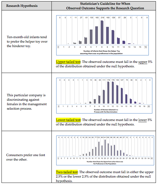
First, note that in our three examples, we examined different parts of the distribution of simulated outcomes when deciding whether the observed study data was extreme. Each of these cases is an example of a specific type of hypothesis test.
Statisticians typically use the following guidelines to determine whether the observed data supports the research question:
Statisticians use what is called a p-value to quantify the amount of evidence that an observed outcome from a set of data provides for a research question.
Making a Decision with p-values
- If the p-value is less than .05 (5%), then the data provide enough statistical evidence to support the research question.
- If the p-value is not less than .05 (5%), then the data do not provide enough statistical evidence to support the research question.
Why does this decision rule work? Consider the “Helper vs. Hinderer” example. Because the p-value falls below 5%, the observed result must have been in the upper 5% of the reference distribution. As stated earlier, this implies that the observed study result is very unlikely to happen by chance under the null hypothesis, which supports the research question.
On the other hand, consider the “Are Women Passed Over for Managerial Training” example. Because the p-value was larger than 5%, the observed result can’t have been in the lower 5% of the reference distribution. This implies that the observed study result is not all that unusual and could have easily happened by chance under the null hypothesis. Therefore, the null hypothesis could be true, and we have no evidence to support the research question.
This decision rule is widely accepted for determining whether study results are statistically significant; however, some researchers do advocate using a more flexible rule similar to the following:
Making a Decision with p-values, Revised
- If the p-value falls below .05, we have strong statistical evidence to support the alternative hypothesis (i.e., the research question).
- If the p-value falls below .10 but above .05, we have “marginal” statistical evidence to support the alternative hypothesis (i.e., the research question).
- If the p-value is above .10, we have no evidence to support the research question.
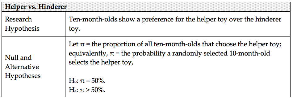
6.1.5. Example 1 - Helper vs. Hinderer?

-
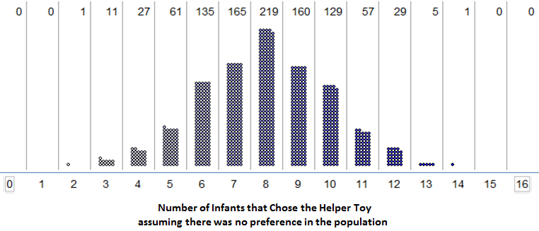
Q-83: Estimate the p-value using the simulation pictured above.
- (A) 0/1000
- Remember that the upper p-value is the percent AT or above the value.
- (B) 1/1000
- This is an upper tail test, so the upper p-value is the fraction of the data that is at 14 (1 out of 1000) and above 14 (0 out of 1000).
- (C) 999/1000
- This is an upper-tail test, use a upper p-value.
- (D) 1000/1000
- This is an upper-tail test, use a upper p-value.
-
Q-84: Based on the p-value from the last question, what is the correct conclusion?
- (A) There is strong evidence supporting the claim that the proportion of the ten-month-old infants tend to prefer the helper toy over the hinderer toy is greater than 50%.
- Since the p-value = 1/1000 = 0.001 < 0.05, we have strong evidence in favor of the alternative hypothesis.
- (B) There is not enough evidence to claim that the proportion of the ten-month-old infants tend to prefer the helper toy over the hinderer toy is greater than 50%.
- A small p-value is always strong evidence in favor of the alternative.
- (C) There is strong evidence supporting the claim that the proportion of the ten-month-old infants tend to prefer the helper toy over the hinderer toy is equal to 50%.
- We never have strong evidence FOR the null hypothesis, only AGAINST the null and for the alternative.
6.1.6. Example 2 - Are Women Passed Over for Managerial Training?

-
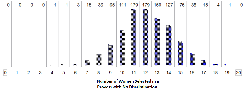
Q-85: Estimate the p-value using the simulation pictured above.
- (A) 56/1000
- Remember that the lower p-value is the percent AT or below the value.
- (B) 121/1000
- This is a lower tail test, so the lower p-value is the fraction at 9 (65 out of 1000) or below 9 (56 out of 1000).
- (C) 879/1000
- This is an lower-tail test, use a lower p-value.
- (D) 944/1000
- This is an lower-tail test, use a lower p-value.
-
Q-86: Based on the p-value from the last question, what is the correct conclusion?
- (A) There is strong evidence supporting the claim that the proportion of women selected is less than 60%.
- A large p-value never strong evidence in favor of the alternative.
- (B) There is not enough evidence to claim that the proportion of women selected is less than 60%.
- The p-value = 121/1000 = 0.121 > 0.05, so we do not have strong evidence in favor of the alternative hypothesis.
- (C) There is strong evidence supporting the claim that the proportion of women selected is equal to 60%.
- We never have strong evidence FOR the null hypothesis, only AGAINST the null and for the alternative.
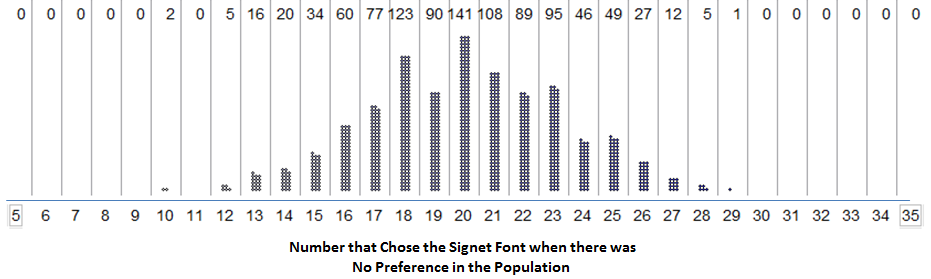
6.1.7. Example 3 - Font Preference?

-
Q-87: Estimate the p-value using the simulation pictured above.
- (A) 0/1000
- The upper p-value is twice the percent of data at or in the direction of the closest tail.
- (B) 1000/1000
- The upper p-value is twice the percent of data at or in the direction of the closest tail.
-
Q-88: Based on the p-value from the last question, what is the correct conclusion?
- (A) There is strong evidence supporting the claim that the proportion of all consumers that select the Signet font is different than 50%
- This is a two-tail test, so the p-value = 2*0 = 0 < 0.05, so there is strong evidence in favor of the alternative hypothesis. In this case, we measure toward the upper tail, then double the value.
- (B) There is not enough evidence to claim that the proportion of all consumers that select the Signet font is different than 50%
- A small p-value is always strong evidence in favor of the alternative.
- (C) There is strong evidence supporting the claim that the proportion of all consumers that select the Signet font is equal to than 50%
- We never have strong evidence FOR the null hypothesis, only AGAINST the null and for the alternative.
6.2. Finding Exact p-values With JMP
6.2.1. Using the Binomial Distribution to Find Exact p-Values
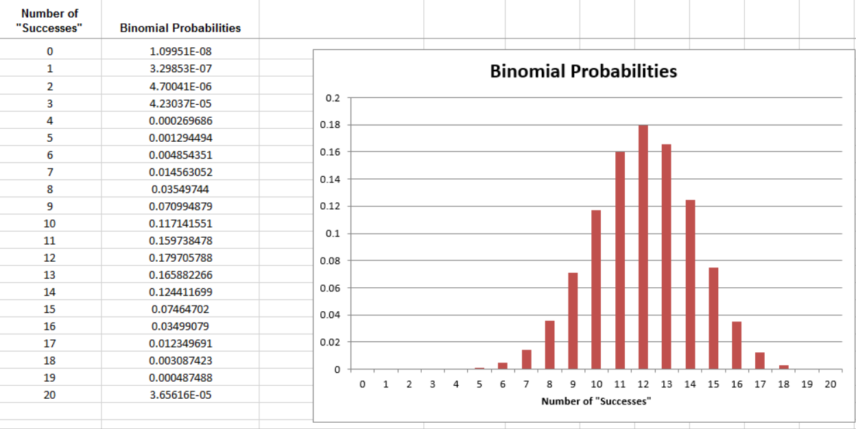
There is one caveat regarding our current approach to obtaining a p-value. Certainly, different simulations will produce slightly different simulated distributions. The general pattern will be the same, but variations do exist. For example, consider the Helper vs. Hinderer study.
The study’s observed result was as follows: 14 out of 16 infants chose the helper toy. What if two different researchers each carried out their own simulation study to estimate the p-value?*
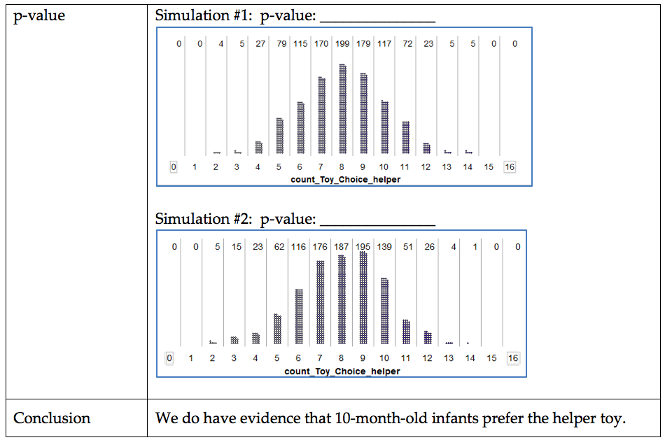
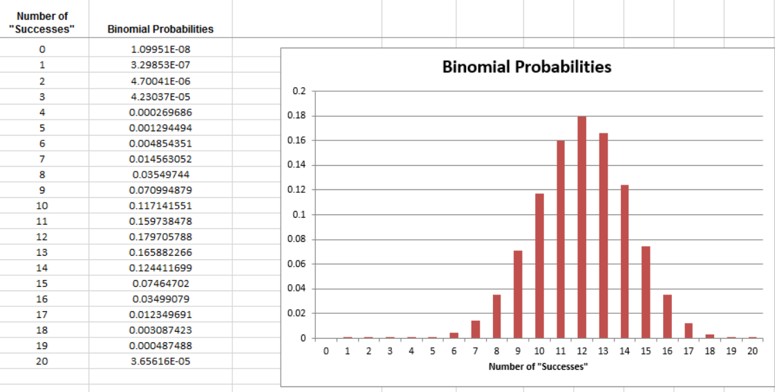
Fortunately, regardless of which simulation study we use in the previous example, the final conclusion is the same, and the discrepancy between the two estimated p-values is minimal; still, it’s not ideal that two different researchers get different results. Note that as the number of trials in our simulation study increases, we expect less discrepancy between these two estimates of the p-value. So, instead of using a simulation study with only 1,000 trials to estimate the p-value, we would ideally like to simulate this experiment over and over again, say an infinite number of times. This would provide us with the theoretical probabilities of interest so that can get exact p-values instead of an estimate of the p-value. The following graphic shows what the distribution would look like if we kept repeating the simulation study over and over again, each time counting and plotting the number of infants that chose the helper toy (assuming there was no real preference in the population of all infants). This theoretical probability distribution is known as the binomial distribution.
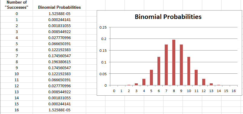
We can calculate these probabilities using the Excel file BinomialProbabilities.xls, which can be found on the course website.
Statisticians often use the binomial distribution to calculate p-values when testing claims about a population proportion. However, before using this distribution, we should check to make sure the following conditions are met (note that these same conditions have to be met in order to estimate the p-value via a simulation study, as well).
The Binomial Distribution - When can we use it?
This distribution can be used whenever the following assumptions are met:
- The study involves a fixed number of trials, n.
- There are only two possible outcomes on each trial (we call these a “success” or “failure”).
- The probability of “success” (π) remains constant from trial to trial.
- The n trials are independent.
Check whether these assumptions seem reasonable for the Helper vs. Hinderer study.
There exist a fixed number of trials, n.
- There are only two possible outcomes on each trial (“success” or
“failure”).
The probability of success (π) remains constant from trial to trial.
The n trials are independent.
6.2.2. Example: Gender Discrimination
Recall that we already estimated the probability of observing 9 or fewer women selected out of 20 if there was no discrimination (i.e., we estimated the p-value with a simulation study).
Estimated p-value = _____________
Next, we will use the binomial distribution to find the exact p-value for the Gender Discrimination Study. First, check whether the assumptions behind the binomial distribution seem reasonable in this case.
There exist a fixed number of trials, n.
- There are only two possible outcomes on each trial (“success” or
“failure”).
The probability of success (π) remains constant from trial to trial.
The n trials are independent.
| Are Women Passed Over for Managerial Training? | |
|---|---|
| Research Hypothesis | The company is discriminating against women when they are selecting employees for management training. |
| Null and Alternative Hypotheses | Let π = the probability the company selects a woman. Ho: π = 60%.
Ha: π < 60%.
|
To find the exact p-value, we will use the binomial distribution with…
p-value: ____________________
Conclusion: We do not have enough evidence that the company is discriminating against females when selecting employees for management training.
6.2.3. Example: Font Preference
Finally, we will use the binomial distribution to find the exact p-value for the Font Preference Study. Recall that we have already estimated this p-value using a simulation study:
Estimated p-value = _____________
Before we use the binomial distribution to find the exact p-value, we will first check whether the assumptions behind the binomial distribution seem reasonable in this case.
There exist a fixed number of trials, n.
- There are only two possible outcomes on each trial (“success” or
“failure”).
The probability of success (π) remains constant from trial to trial.
The n trials are independent.
| Font Preference Study | |||||||||||||||||||||||||||||||||||||||||||||||||||||||||||||||||||||||||||||||||||||
|---|---|---|---|---|---|---|---|---|---|---|---|---|---|---|---|---|---|---|---|---|---|---|---|---|---|---|---|---|---|---|---|---|---|---|---|---|---|---|---|---|---|---|---|---|---|---|---|---|---|---|---|---|---|---|---|---|---|---|---|---|---|---|---|---|---|---|---|---|---|---|---|---|---|---|---|---|---|---|---|---|---|---|---|---|---|
| Research Hypothesis | Consumers prefer one font over the other. | ||||||||||||||||||||||||||||||||||||||||||||||||||||||||||||||||||||||||||||||||||||
| Null and Alternative Hypotheses | Let π = the proportion of all consumers that would choose the Signet font; equivalently, let π = the probability of a randomly selected consumer choosing the Signet font. Ho: π = 50%. Ha: π ≠ 50%. | ||||||||||||||||||||||||||||||||||||||||||||||||||||||||||||||||||||||||||||||||||||
| p-value | To find the exact p-value, we will use the binomial distribution with… n = ________ and π = _______
|
||||||||||||||||||||||||||||||||||||||||||||||||||||||||||||||||||||||||||||||||||||
| Conclusion | There is evidence that consumers have a preference towards one font over the other (more chose the Signet font). |
6.2.4. Using JMP to Find p-values for the Binomial Exact Test
6.2.5. Analyzing a Distribution with Raw Data
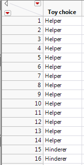
Earlier, we used Excel to calculate binomial probabilities and to find the p-value associated with the binomial exact test. This test is also easily implemented in JMP when given the raw data. For example, the data from the Helper/Hinderer example could be entered into JMP as follows:
To get the test statistic and p-value in JMP, select Analyze > Distribution. Enter the following:
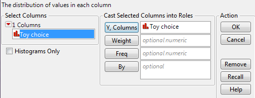
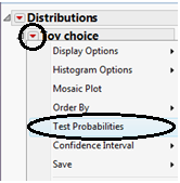
On the output that appears, select “Test Probabilities” from the red drop-down arrow next to the variable name:
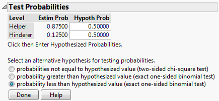
Enter the following:
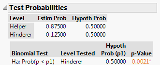
Click “Done” and JMP should return this output:
6.2.6. An Alternative Method of Setting up the Data Sheet
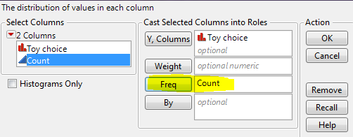
You can also set up the data as shown below:

If you provide the summarized data to JMP as shown above, then enter the following after selecting Analyze > Distribution:
From here on out, the steps are the same as shown on the previous page.
On the output that appears, select “Test Probabilities” from the red drop-down arrow next to the variable name:
Enter the following:
Click “Done” and JMP should return this output:
-
Q-89: What is the p-value in the picture shown above?
- (A) 0.8750
- Look in the bottom right part of the picture.
- (B) 0.1250
- Look in the bottom right part of the picture.
- (C) 0.5000
- Look in the bottom right part of the picture.
- (D) 0.0021
-
Q-90: Is the statistic unusually large? Why?
- (A) Yes, since the p-value is less than 0.05 (5%).
- Small p-values mean unsual values!
- (B) No, because the p-value is no large enough.
- Small p-values mean unsual values!
-
Q-91: What is the correct conclusion in this case?
- (A) There is strong evidence supporting the claim that the infants prefer the helper toy.
- Since it would be rare to get a statistic this large when there is no preference, we are confident that the infant DO prefer the helper toy.
- (B) There is not enough evidence to claim that the infants prefer the helper toy.
- Since it would be rare to get a statistic this large when there is no preference, we are confident that the infant DO prefer the helper toy.
6.3. More Information About Hypothesis Tests
6.3.1. More on Using p-Values to Make Decisions
As mentioned earlier, some researchers advocate using the following guidelines:
p-Value Guidelines
- If the p-value falls below .05, there is strong evidence to support the research hypothesis.
- If the p-value falls below .10 but above .05, there is “marginal” evidence to support the research hypothesis.
- If the p-value is above .10, there is not enough evidence to support the research hypothesis.
In general, the smaller the p-value, the less likely the results of the study are due to random chance; thus, the more evidence we have that to support the research hypothesis. In some disciplines, the p-value must be much smaller than .05 in order to support a research hypothesis. For example, physics journals often like to see p < .001. Though the above guidelines allow for claims of “marginal” evidence when p-values fall between .05 and .10, some statisticians caution against this. For example, Irwin Bross argues that such modifications would be detrimental in evaluating evidence.
Anyone familiar with certain areas of the scientific literature will be well aware of the need for curtailing language-games. Thus if there were no 5% level firmly established, then some persons would stretch the level to 6% or 7% to prove their point. Soon others would be stretching to 10% and 15% and the jargon would become meaningless. Whereas nowadays a phrase such as statistically significant difference provides some assurance that the results are not merely a manifestation of sampling variation, the phrase would mean very little if everyone played language-games. To be sure, there are always a few folks who fiddle with significance levels–who will switch from two-tailed to one-tailed tests or from one significance test to another in an effort to get positive results. However, such gamesmanship is severely frowned upon.
Source:
Bross IDJ (1971), “Critical Levels, Statistical Language and Scientific Inference,” in Foundations of Statistical Inference.
The “.05 rule” is usually attributed to R.A. Fisher. His published thoughts on the matter are given below.
In the investigation of living beings by biological methods statistical tests of significance are essential. Their function is to prevent us being deceived by accidental occurrences, due not to the causes we wish to study, or are trying to detect, but to a combination of the many other circumstances which we cannot control. An observation is judged significant, if it would rarely have been produced, in the absence of a real cause of the kind we are seeking. It is a common practice to judge a result significant, if it is of such a magnitude that it would have been produced by chance not more frequently than once in twenty trials. This is an arbitrary, but convenient, level of significance for the practical investigator, but it does not mean that he allows himself to be deceived once in every twenty experiments. The test of significance only tells him what to ignore, namely all experiments in which significant results are not obtained. He should only claim that a phenomenon is experimentally demonstrable when he knows how to design an experiment so that it will rarely fail to give a significant result. Consequently, isolated significant results which he does not know how to reproduce are left in suspense pending further investigation.
Source:
R.A. Fisher (1929), “The Statistical Method in Psychical Research,” from the* Proceedings of the Society for Psychical Research*, 39, 189-191. *
6.3.2. Examining the Effect of Sample Size
Example 2.3: Gender Discrimination, Revisited
Once again, consider the Gender discrimination example. Recall that of the 20 persons selected for management so far, only 9 (or 9/20 = 45%) were female. In an unbiased selection process, we expected to see a woman selected 60% of the time. We found that the probability of observing 9 or fewer women selected by chance if the company was in fact using a fair selection process was .1275.
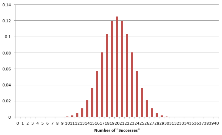
Now, suppose that the results had actually been as follows: Of the last 40 persons selected for management so far, only 18 (or 18/40 = 45%) were female. How does this change the calculation of the p-value? The binomial probabilities for this scenario are shown below.
| Number of “Successes” | Binomial Probabilities |
|---|---|
| 0 | 1.20893E-16 |
| 1 | 7.25355E-15 |
| 2 | 2.12166E-13 |
| 3 | 4.03116E-12 |
| 4 | 5.59324E-11 |
| 5 | 6.0407E-10 |
| 6 | 5.28561E-09 |
| 7 | 3.85094E-08 |
| 8 | 2.38277E-07 |
| 9 | 1.27081E-06 |
| 10 | 5.90928E-06 |
| 11 | 2.41743E-05 |
| 12 | 8.76319E-05 |
| 13 | 0.000283118 |
| 14 | 0.000819021 |
| 15 | 0.002129454 |
| 16 | 0.004990908 |
| 17 | 0.010568983 |
| 18 | 0.020257217 |
| 19 | 0.035183587 |
| 20 | 0.055414149 |
| 21 | 0.07916307 |
| 22 | 0.102552159 |
| 23 | 0.120387317 |
| 24 | 0.127911524 |
| 25 | 0.122795063 |
| 26 | 0.106264959 |
| 27 | 0.082650523 |
| 28 | 0.057560186 |
| 29 | 0.035727012 |
| 30 | 0.019649857 |
| 31 | 0.009507995 |
| 32 | 0.004011185 |
| 33 | 0.001458613 |
| 34 | 0.000450454 |
| 35 | 0.000115831 |
| 36 | 2.41315E-05 |
| 37 | 3.91321E-06 |
| 38 | 4.63406E-07 |
| 39 | 3.56467E-08 |
| 40 | 1.33675E-09 |
For this scenario, the p-value is given by ______________.
Finally, we can also consider a third study in which of the last 200 persons selected for management so far, only 90 (or 90/200 = 45%) were female. How would you find the p-value for this scenario?
For this scenario, the p-value is given by ______________.
Recall that these binomial distributions give us an idea of what outcomes occur by chance when the selection process does not discriminate based on gender (because we used π = 60%).
| Study #1: | n = 20 trials Observed Result = 9/20 = 45% |
|---|---|
| Study #2: | n = 40 trials Observed Result = 18/40 = 45% |
| Study #3: | n = 200 trials Observed Result = 90/200 = 45% |
Question:
Which of the following statements is most correct?
- The three studies provide equally convincing statistical evidence that the selection process discriminates against women.
- Study #1 provides the most convincing statistical evidence that the selection process discriminates against women.
- Study #2 provides the most convincing statistical evidence that the selection process discriminates against women.
- Study #3 provides the most convincing statistical evidence that the selection process discriminates against women.
Explain your reasoning.
6.3.3. Practical Significance versus Statistical Significance
Consider the previous example. As discussed earlier, the result in Study #1 is not “statistically significant” because the observed outcome does not fall in the bottom 5% of simulated outcomes (i.e., the p-value is not below .05). On the contrary, the results in Study #2 and Study #3 are “statistically significant.” The previous example illustrates that statistical significance depends on the sample size.
All three studies resulted in an outcome of 45% of those selected for management being female, but this result was only statistically significant in the studies with the larger sample size. This presents a conundrum: If a study’s results are not statistically significant, it could be that the effect under study is real, but the sample size wasn’t large enough to detect that effect (this relates to a concept known as the power of a hypothesis test which is discussed in upper-level statistics courses). On the other hand, if the sample size is large enough, very small differences between the observed results and the expected value in the null hypothesis can lead to statistically significant differences.
To counter this, researchers often consider “practical significance” in addition to “statistical significance.” A result is known as “practically significant” if the difference between the observed and expected result is large enough to be of value in the practical sense.
6.3.4. Example 2.4: Dukes vs. Wal-mart Stores, Inc.
The lead plaintiff in this case, Betty Dukes, was a Wal-Mart employee. She and others alleged gender discrimination in promotion policies and practices in Wal-Mart stores.
As the nation’s largest private employer, Wal-Mart makes tens of thousands of promotion decisions each year. The following data was provided during this trial: Wal-Mart promoted roughly 50,000 individuals to management between 1997 and 2002. Female employees constituted about 60% of the group eligible for these promotions.
Questions:
How many of the 50,000 individuals promoted do you expect to be female if Wal-Mart is not discriminating based on gender?
Suppose that 29,780 of the individuals promoted were women (note that this was not the actual outcome in the court case). What percentage is this?
A simulation study with 100 trials was conducted to see what outcomes occur by chance when the selection process is not discriminatory. The results are shown below.
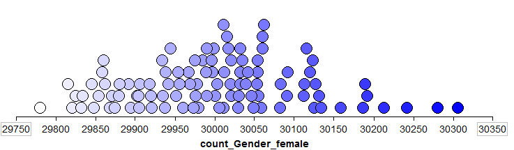
Recall the hypothetical observed value of 29,780 females being selected. The research hypothesis is that Wal-Mart is discriminating against women in their promotion policies and practices. Based on the results of the simulation study, is this result “statistically significant”? Explain.
In the previous question, you estimated the p-value for this research hypothesis. Use the binomial distribution to find the exact p-value. Again, is the result “statistically significant”?
Is this result “practically significant”? Explain.
Do you foresee any problems if we rely on only statistical significance when making decisions? Explain.
6.4. Confidence Interval for a Proportion
When carrying out hypothesis tests, we are testing claims about population parameters. Sometimes, however, our goal is to estimate a parameter of interest. Statisticians typically do this with a confidence interval, which is simply a range of likely values for the parameter of interest. The big difference between hypothesis testing and confidence intervals is as follows: the construction of a confidence interval does NOT require any hypotheses concerning our population parameter of interest.
6.4.1. Example 2.5: Star Tribune Poll Regarding Legalization of Medical Marijuana
In February of 2014, a Star Tribune Minnesota poll asked a random sample of adults in Minnesota, “Do you support or oppose legalizing marijuana for medical purposes in Minnesota?” Of the 800 adults surveyed, 408 (51%) answered that they would support this.

Source: http://www.startribune.com/politics/statelocal/245910931.html
Questions:
Ultimately, the Star Tribune conducted this poll because they wanted to estimate the proportion of adults in Minnesota that felt (at the time of the survey) that medical marijuana should be legalized. Keep this in mind as you answer the following questions.
- What is the population of interest?
- What is the parameter of interest?
- What is the sample?
- What is the sample statistic of interest?
Based on the results of this poll, our best guess for the proportion of all Minnesotans that feel medical marijuana should be legalized is = 408/800 = 51%. This is called a point estimate.
We know, however, that if a different sample of 800 Minnesotan adults had been polled, this point estimate would likely change. So, instead of using only this point estimate, we’ll also use statistical methods to estimate the parameter of interest with a range of likely values (this range is called the confidence interval). To get this range of likely values, we’ll start with our point estimate (i.e., the sample statistic, = 51%). This is our best guess so far. Then, we can use Tinkerplots to get an idea of how much we expect this statistic to change from one random sample to the next because of natural sampling variation. The distribution of sample proportions obtained by repeated sampling is shown below.
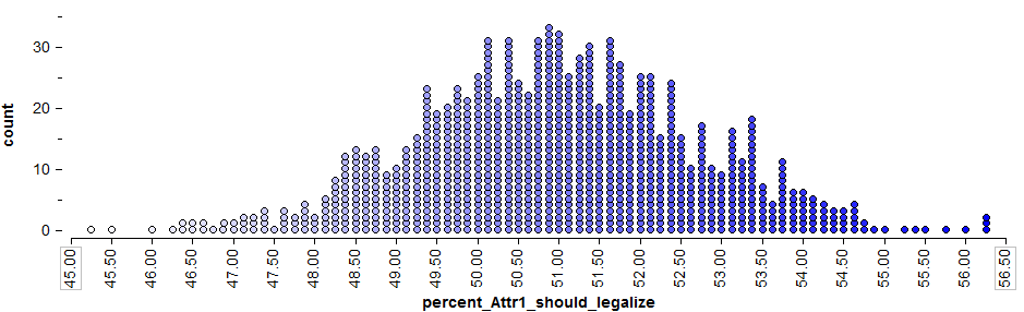
To get a 95% confidence interval for the parameter of interest, we find both the lower endpoint and the upper endpoint that separate the “middle” 95% of this distribution from the outer 5%.
Questions:
- Find the lower and upper endpoints for a confidence interval for the parameter of interest, π = the proportion of all Minnesotan adults that felt medical marijuana should be legalized.
- Interpret this confidence interval.
6.4.2. Confidence Intervals with StatKey
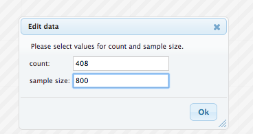
In StatKey’s Confidence Interval for a Single Proportion , we need to enter the statistic by clicking Edit Data and entering the statistic, as shown below.
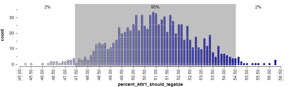
Then, we can use StatKey to get an idea of how much we expect this statistic to change from one random sample to another. Similar to the TinkerPlots simulation, the distribution of sample proportions obtained by repeated sampling is shown below.
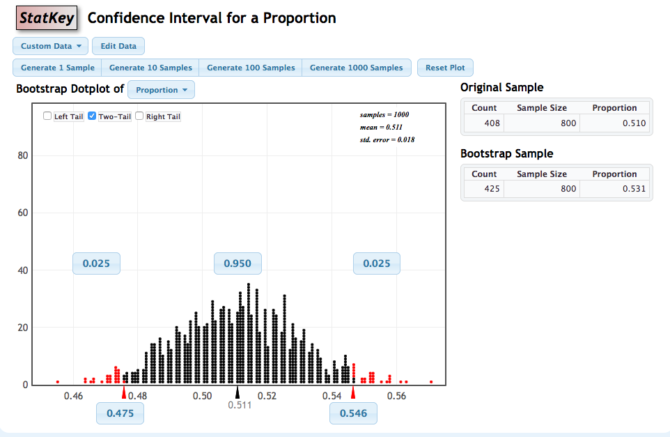
To get a 95% confidence interval for the parameter of interest, we find both the lower endpoint and the upper endpoint that separate the “middle” 95% of this distribution from the outer 5%. As before, this is accomplished by clicking two-tail and setting the confidence level to the desired value.
Note
As before, you should always report your confidence interval in a well-formed sentence that describes the parameter of interest in the context of the problem. For example, for the intervals shown above, we would write
We are 95% confidence that the population proportion of all Minnesotans that feel medical marijuana should be legalized is between 0.475 and 0.546
Note that we are trying to estimate the value for the whole population, not the sample.
6.4.3. Confidence Intervals in JMP
Note that we could also use JMP to find this confidence interval. JMP uses what is known as the score method instead of Wald’s method, which would be more appropriate in this case.

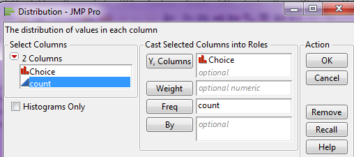
Select Analyze > Distribution and enter the following:
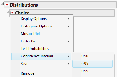
Then, click the red drop-down arrow next to the variable name (in this case “Choice”) and select Confidence Interval > .95.
JMP returns the following:
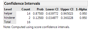
Interpret this confidence interval.
Note
The hypothesis test for this problem provided evidence that the true population parameter was greater than 50%. The confidence interval tells us this and more…
HOW MUCH GREATER it is!