Summarizing Data
Next, we will present some basic methods for summarizing a distribution, both numerically and graphically.
Graphing Distributions - Dot Plots and Histograms
Shapes of a Distribution
One of the important features of a distribution is the shape of the distribution. In this class, we will describe the shape of the distribution in words using terms like symmetric, skewed left, skewed right, and bimodal.
- Symmetric
- A distribution is described as symmetric if portion of the graph to the left of the mean/average is approximately a mirror image of the portion of the graph to the right side of the mean/average.
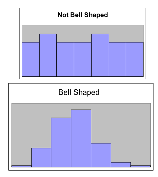
We will distinguish between symmetric graphs that are bell-shaped or not bell-shaped.
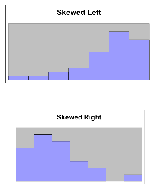
On the other hand, when a distribution is not symmetric, we focus on the tails of the distribution.
- Skewed Left
- A distribution is skewed left when it has a long left tail, that is its left tail is much longer than its right tail.
- Skewed Right
- A distribution is skewed right when it has a long right tail, that is its right tail is much longer than its left tail.
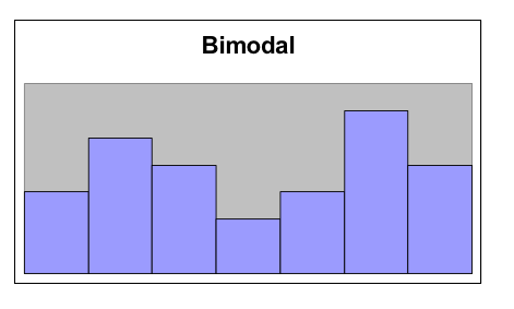
Finally, it is possible that we might have a graph with two peaks.
- Bimodal
- A distribution is bimodal if it has two distinct peaks. (The term bimodal literally means two modes, where a mode is a peak.)
-
Q-48: A distribution with two similar tails is ...
- (A) Symmetric
- A symmetric graph has two tails that are about the same.
- (B) Skewed left
- A skewed left graph has a longer left tail.
- (C) Skewed right
- A skewed right graph has a longer right tail.
-
Q-49: A distribution with long left tail is ...
- (A) Symmetric
- A symmetric graph has two tails that are about the same.
- (B) Skewed left
- A skewed left graph has a longer left tail.
- (C) Skewed right
- A skewed right graph has a longer right tail.
-
Q-50: A distribution with long right tail is ...
- (A) Symmetric
- A symmetric graph has two tails that are about the same.
- (B) Skewed left
- A skewed left graph has a longer left tail.
- (C) Skewed right
- A skewed right graph has a longer right tail.
Measures of Center - Finding a Typical Value
- Mean or Average
- This is the (arithmetic) average of the data. It is calculated by all the values of the variable and dividing by the number of individuals.
- Median
- A value that splits the data into groups that consist of approximately half of the data. It is computed by (1) Putting the data in order and (2) Finding the middle value. If the data set has an even number of values, the average of the middle two values is used for the median.
While being able to compute the value of a summary statistic is important, *it is even more important to understand what each number tells us about the distribution. Here are the standard interpretations for these statistics.
Standard Interpretation of the Mean
The mean is the balance point or center of mass of the distribution, that is, it is the location at which the dot plot would balance on your finger.
Standard Interpretation of the Median
The median splits the data in half. Approximately 50% of the data will be above and below the median. (The only situation where this is not exactly 50% is when there are multiple values stacked at the median.)
- (A) 252.0
- You need to add up all the values and divide by the number of individuals.
- (B) 283.0
- You need to add up all the values and divide by the number of individuals.
- (C) 293.8
Q-51: The following values are the serum cholesterol levels (mg/dLi) of six men with high cholesterol.
366 327 230 274 292 274
Compute the mean of these data.
- (A) 252.0
- Make sure you reorder the data, *then* find the middle value.
- (B) 283.0
- (C) 293.8
- Sort the data and find the middle value.
Q-52: The following values are the serum cholesterol levels (mg/dLi) of six men with high cholesterol.
366 327 230 274 292 274
Compute the median of these data.
Unusual Values and the p-Value
We will spend a considerable amount of time in this course trying to decide if a value is unusually large or unusually small. For example, if we were trying to determine if the hiring practices in a school district are discriminatory, we will need to determine if the school hires an unusually low number of African-American teachers.
Before we can determine if a value is unusual, we need a good definition of what it means to be unusually large or unusually small in a statistical sense.
- Unusually large values
- A value is considered unusually large if it is in the largest 5% of the distribution.
- Unusually small values
- A value is considered unusually small if it is in the smallest 5% of the distribution.
Note
There is nothing special about picking 5%, and in fact later in the course we will see that adjusting this value gives us some control over a certain type of error. For now, we will stick to 5% and call this the 5% rule.
Now that we know what it means to be unusually large or small, we need a method of determining if a specific value of interest is unusually large. For example, I have a friend that is 78 inches tall (6’ 6”). I know that he is fairly tall, but is he unusually tall, in the statistical sense?
When answering this question intuitively, I believe that it is natural to compare my friend to other tall people, asking What percentage of the time do I meet men that is 78 inches tall or taller. This is the exact intuition that leads to our definition of an upper p-value.
On the other side of the coin (or in this case distribution), we might ask if someone that is 63.5 inches tall, like my wife, is unusually short. Again in a statistical sense. This time it is natural to compare someone on the small side of the distribution with other small values, leading to what I like to call a lower p-value.
- Upper p-value
- The upper p-value of a given value x is the proportion of the distribution that is at or above the value. This measurement is useful in determining if a value is unusually large.
- Lower p-value
- The lower p-value of a given value x is the proportion of the distribution that is at or below the value. This measurement is useful in determining if a value is unusually small.
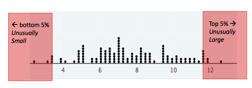
Example: Using a lower p-value to determine if 4 is unusually small.
Consider the distribution shown below. There are 117 dots on the graph, and we want to answer the question Is the value 4 unusually small. Because we are focusing on small values, we will use a lower p-value, because it makes sense to compare a potentially small value to other small values. There are 7 dots that are at or below 4, so the lower p-value of 4 rounds up to 0.06 or 6%. Since there is more than 5% of the distribution below 4, 4 is not in the smallest 5% of the distribution and therefore is not unusually small.
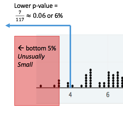
Thus, a value is only unusually small if its lower p-value is smaller than 5% (when using the 5% rule). The same is true for an upper p-value.
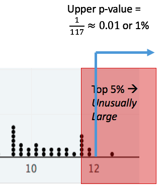
Example: Using an upper p-value to determine if 12 is unusually large.
This time, consider the question Is 12 unusually large? In this case the upper p-value is a little less than 1%. Since less than 5% of the distribution is above 12, we see that
- 12 is in the largest 1%, and
- 12 is unusually large, according to the 5% rule.
-
Q-53: When deciding if a value is unusually small, use a ...
- (A) lower p-value.
- When looking at a potentially small value, compare it to other small values.
- (B) upper p-value.
- Focus on the smallest part of the distribution, i.e. the left tail.
-
Q-54: When deciding if a value is unusually large, use a ...
- (A) lower p-value.
- Focus on the largest part of the distribution, i.e. the right tail.
- (B) upper p-value.
- When looking at a potentially large value, compare it to other large values.
-
Q-55: Suppose that a value has a lower p-value of 2.3%. According to the 5% rule, is this value unusually small?
- (A) Yes
- If the lower p-value is smaller than 5%, the value is in the smallest 5% and thus unusually smallest.
- (B) No
- Consider the fact that the value has only 2.3% of the distribution below it. Is it in the smallest 5% of the distribution?
-
Q-56: Suppose that a value has an upper p-value of 12.7%. According to the 5% rule, is this value unusually large?
- (A) Yes
- Consider the fact that the value more than 12.7% of the distribution above it. Is it in the largest 5% of the distribution?
- (B) No
- If the upper p-value is larger than 5%, the value is NOT in the largest 5% and thus NOT unusually large.
General P-value Rule
A value is unusually small when the lower p-value is less than 5% (when using the 5% rule).
A value is unusually large when the upper p-value is less than 5% (when using the 5% rule).
In both cases, small p-values mean unusual values.
Measures of Spread - Finding the Amount of Concentration or Spread
In an earlier section, we took on the task of determining a value for a “typical value”. The answer was to use a measurement in the center of the distribution of like the mean and median. Unfortunately, knowing the location of the center of the distribution is not enough information.
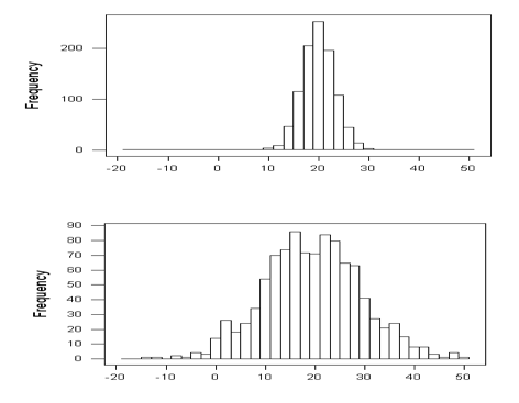
For example, the two graphs shown above have centers that are very similar, but one graph has data that is more concentrated than another. This difference is very important in many fields. In manufacturing, creating products that are very similar can reduce waste, and in statistics, having estimates that are more concentrated, or less spread out, means that we are making better guesses.
The most basic measurement of spread is the range of the data.
- Range
- The difference/distance between the largest and smallest value in the data set.
Unfortunately, the range is very susceptible to outliers, making it a poor measure of spread. We will instead use two other measures of spread, the .. mchoice:
:answer_a: The difference between the smallest and largest values in the data.
:answer_b: The distance between a typical/average value and the mean.
:answer_c: The the range of the middle 50% of the data.
:correct: b

The standard deviation can be through of as ...
interquartile range (IQR) and the standard deviation (from the mean).
- Interquartile range (IQR)
- The range of the middle 50% of the data. It is found by (a) finding the medians of the lower and upper halves of the data, called Q1 and Q3, respectively. Then the IQR = Q3 - Q1.
- Standard Deviation (SD)
- The standard deviation is computed using the formula given below. It can be thought of as the distance of a typical/average value to the mean.
For both statistics, the value tells us how concentrated or spread out the data is.
- A larger value of the SD or IQR means that the data is more spread out.
- A smaller value of the SD or IQR means that the data is more concentrated.
As before, understanding how to interpret the value of a statistic is perhaps more important than being able to compute the value. Here are the standard interpretations of each of these statistics.
Standard Interpretation of the Standard Deviation
The standard deviation tells us how far a typical value is from the mean.
Standard Interpretation of the Interquartile Range
The interquartile range measures the spread of the middle 50% of the data.
Resistance
The IQR is more resistant to the effects of outliers than the standard deviation.
-
Q-57: The standard deviation can be thought of as ...
- (A) The difference between the smallest and largest values in the data.
- (B) The distance between a typical/average value and the mean.
- (C) The range of the middle 50% of the data.
-
Q-58: The interquartile range can be through of as ...
- (A) The difference between the smallest and largest values in the data.
- (B) The distance between a typical/average value and the mean.
- (C) The range of the middle 50% of the data.